AMA Manual of Style - Stacy L. Christiansen, Cheryl Iverson 2020

Figures
Tables, Figures, and Multimedia

The term figure refers to any graphical display used to present information or data,⁴ including statistical graphs, maps, matrixes, algorithms, illustrations, digital images, photographs, and other clinical images. Figures may be used to clarify or explain methods, to present evidence and quantitative results, to highlight trends and associations or relationships among data, to clarify complex concepts, or to illustrate items or procedures. Figures should be accurate, clear, and concise. As with tables, the figure with its title and legend should be understandable without undue reference to the text.

In scientific articles, the choice of a particular type of figure depends on the purpose and type of information being displayed. Some of the most common types of figures in biomedical publications are discussed herein.

4.2.1 Statistical Graphs.

4.2.1.1 Line Graphs.

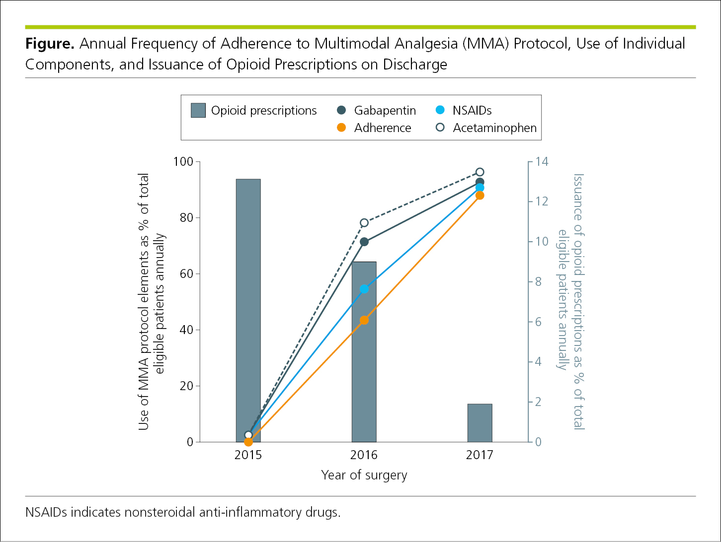
Line graphs have 2 or 3 axes with continuous scales on which data points connected by curves show the association or relationship between 2 or more variables, such as changes over time. In general, line graphs are not ideal for displaying values where connection between points would imply continuity that may not be in evidence.⁷ Line graphs usually are designed with the dependent variable on the vertical axis (y-axis) and the independent variable on the horizontal axis (x-axis).⁴ If justified, a secondary vertical axis⁸ may be used to display an additional set of data (Figure 4.2-1 and Figure 4.2-2) (see 4.2.6.1, Components of Figures, Scales for Graphs).

Figure 4.2-1. Graph With the Dependent Variable on the Vertical Axis (y-Axis) and the Independent Variable on the Horizontal Axis (x-Axis)

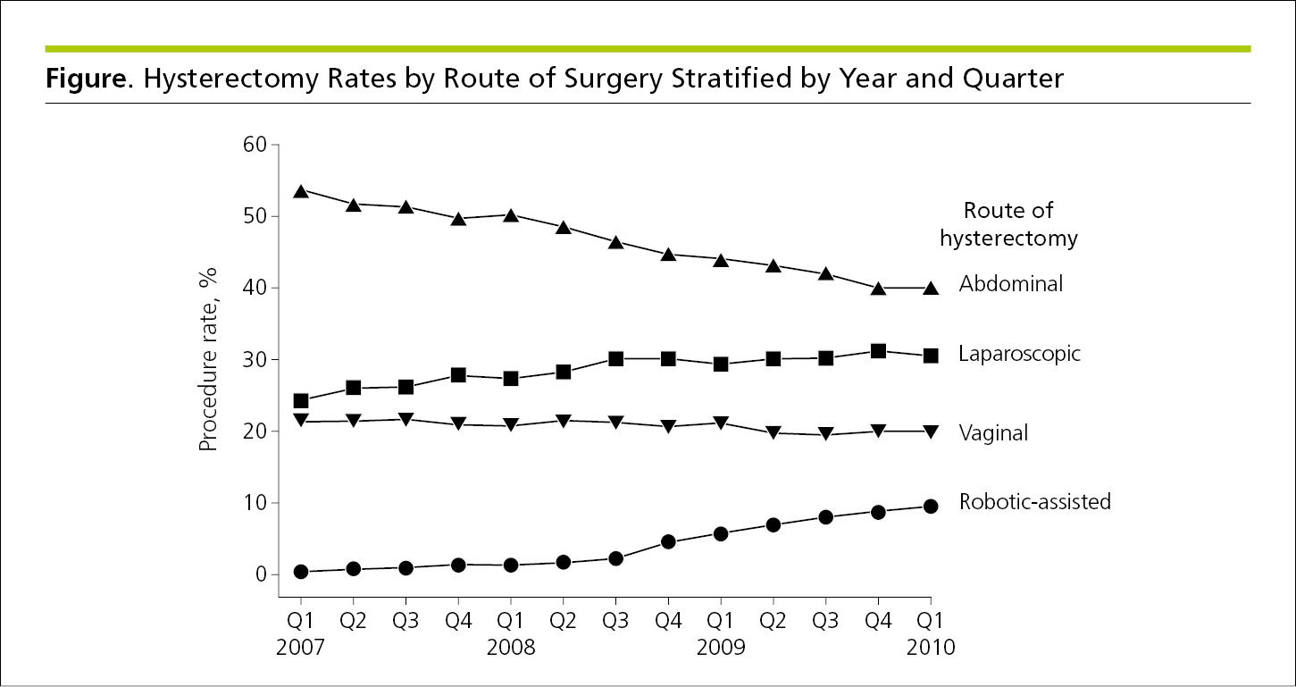
Figure 4.2-2. Graph With 3 Axes (an x-Axis, a y-Axis, and a Secondary y-Axis) to Facilitate Comparison of Related Data

Axes should be continuous; broken axes disrupt any correlation between the large and small values, and the data are not easy to compare. Tick marks provide reference for points on a scale. Each tick mark represents a specified number of units on a continuous scale or the value of a category on a categorical scale. Tick marks should project to the outside of the graph, and intervals between tick marks in general should be regular and predictable to avoid confusion. Data markers should align with ticks, not fall between them. When relevant, show variability of data points in both directions and ensure that what the variability represents (eg, 95% CI) is identified (see 4.2.6.3, Components of Figures, Error Bars).

4.2.1.2 Survival Plots.

Survival plots of time-to-event outcomes, such as those from Kaplan-Meier survival analyses, display the proportion or percentage of individuals, represented on the y-axis, remaining free of or experiencing a specific outcome over time, represented on the x-axis. When the outcome of interest is relatively frequent (eg, occurs in approximately ≥70% of the study population), event-free survival may be plotted on the y-axis from 0 to 1.0 (or 0% to 100%), with the curve starting at 1.0 (100%). When the outcome is relatively infrequent (eg, occurs in <30% of the study population), it may be preferable to plot upward starting at 0 so that the curves, which plot cumulative incidence,^9,10 can be seen without breaking or truncating the y-axis scale (Figure 4.2-3).¹¹ The curve should be drawn as a step function (not smoothed), and the y-axis label should specify the outcome plotted (eg, survival or disease recurrence).

Figure 4.2-3. Survival Curves Showing Time-to-Event Outcomes Plotted Downward (Top) or Upward (Bottom), Depending on the Frequency of the Occurrence (Variable of Interest)

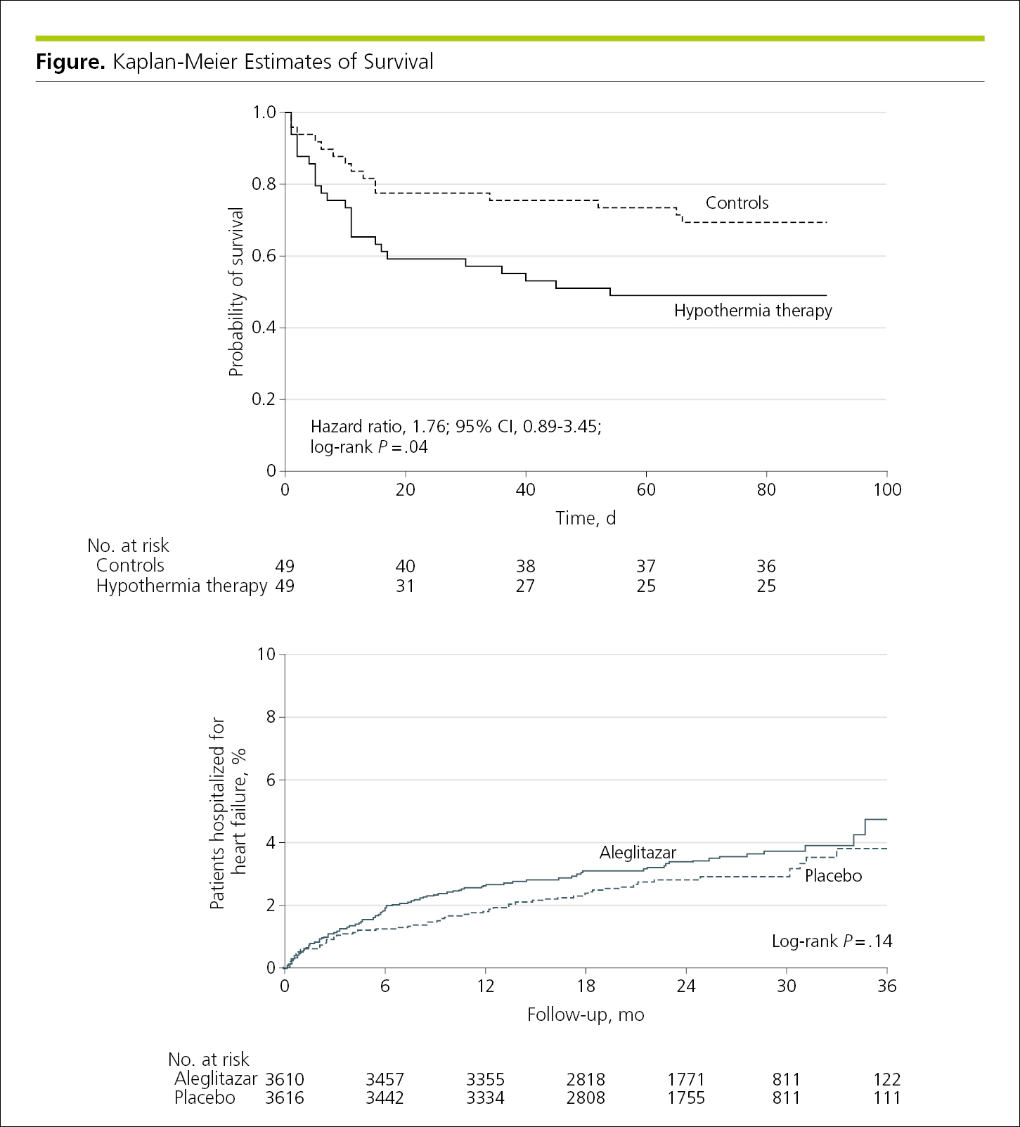
The number of individuals included in the analysis at each interval (number at risk) should be shown underneath the x-axis. Time-to-event estimates become less certain as the number of individuals diminishes, so consideration should be given to not displaying data when less than 20% of the study population is still in follow-up.¹¹ Plots should include some indication of statistical uncertainty, such as error bars on the curves at regular time points or, when time-to-event data are being compared for 2 or more groups, an overall estimate of treatment difference, such as a relative risk (with 95% CI) or log-rank P value. This information can be placed within the graph (Figure 4.2-3).

4.2.1.3 Scatterplots.

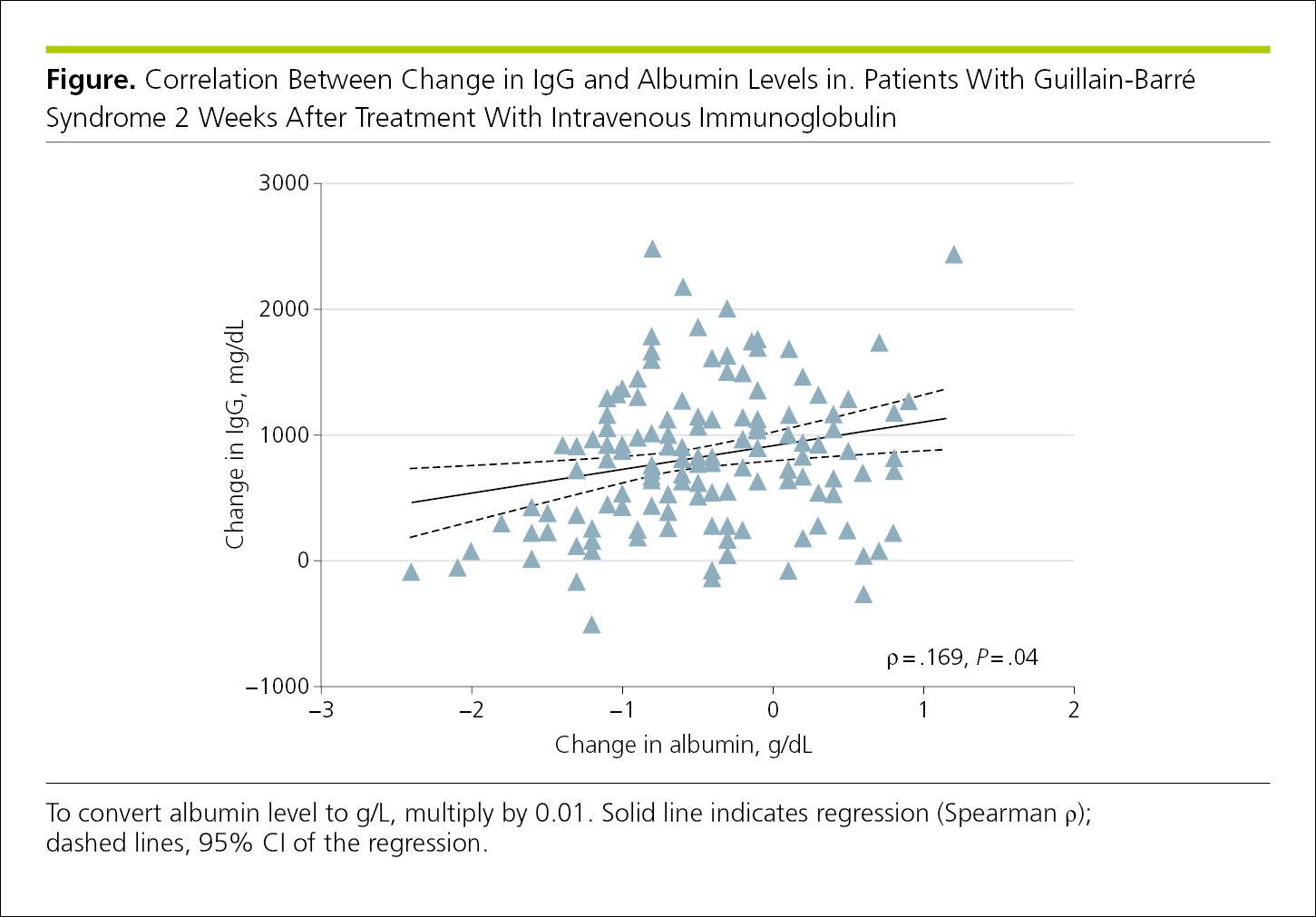
Scatterplots, graphs that represent bivariate data as points on a 2-dimensional Cartesian plane,¹² are useful to convey an overall impression of the relationship between 2 variables.⁷ In scatterplots, individual data points are plotted according to coordinate values with continuous x- and y-axis scales. By convention, independent variables are plotted on the x-axis and dependent variables on the y-axis. Data markers are not connected by a curve, but a curve that is generated mathematically may be fitted to the data (not connecting any points but drawn through “the center”) to summarize the relationship among the variables. The statistical method used to generate the curve and the statistic that summarizes the relationship or association between the dependent and independent variables, such as a correlation or regression coefficient, should be provided in the figure or legend along with the sample size, the P value for the slope of the line, and some indication of how the P value was derived¹ (Figure 4.2-4).

Figure 4.2-4. Scatterplot With the Regression Line, Correlation Statistic, and PValue in the Plot

4.2.1.4 Histograms and Frequency Polygons.

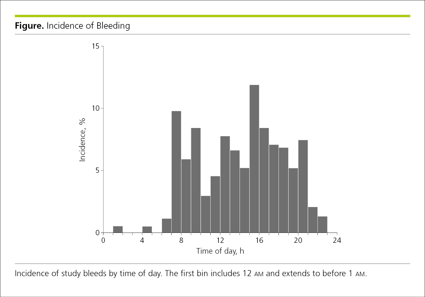
Histograms and frequency polygons display the distribution of data in a data set by plotting the frequency (count or percentages) of observations (on the y-axis) for each interval represented on the x-axis. In both histograms and frequency polygons, the y-axis must begin at 0 and should not be broken, and the x-axis is a continuous, quantitative scale. Histograms are plotted with continuous bars of equal width determined by the x-axis intervals, in which bar height represents frequency (counts or percentages) so long as the bars are of equal width. For additional detail on these statistics, see Haighton et al.¹³ No spacing is used between bars—they are either closed up or separated with a very thin white line (Figure 4.2-5).

Figure 4.2-5. Histogram Showing Frequencies for Each Period (Bar Height Represents Percentage of Cases)

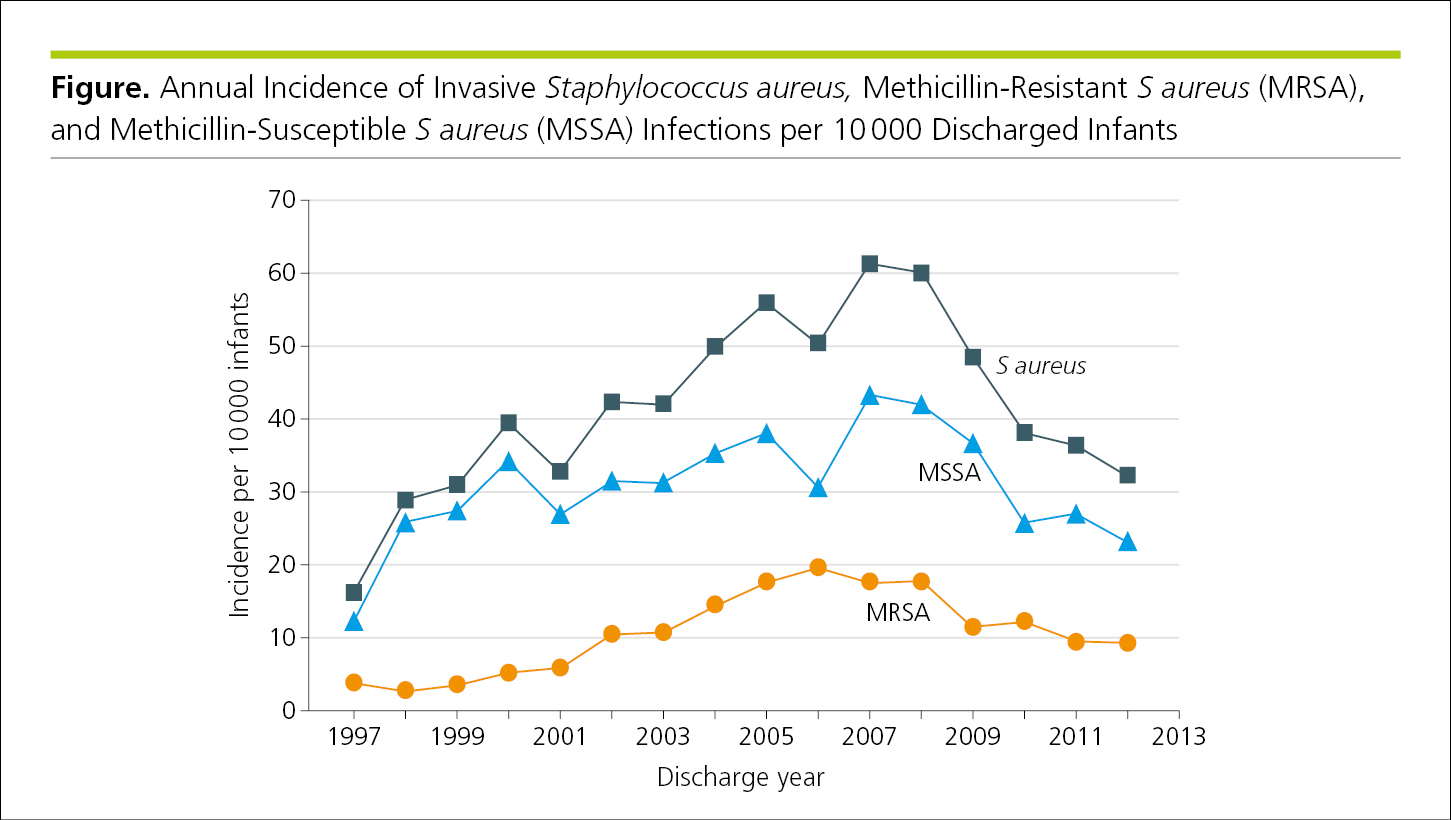
Frequency polygons use data markers (representing the tops of the columns of a histogram) to represent frequency connected by a curve. Data distributions from multiple data sets that overlap can be plotted in a frequency polygon but not in a histogram (Figure 4.2-6). A frequency polygon (or histogram) is used to display the entire frequency distribution (counts) of a continuous variable.

Figure 4.2-6. Frequency Polygons Can Illustrate Distributions for Multiple Groups or, as in This Figure, Infection Types

4.2.1.5 Bar Graphs.

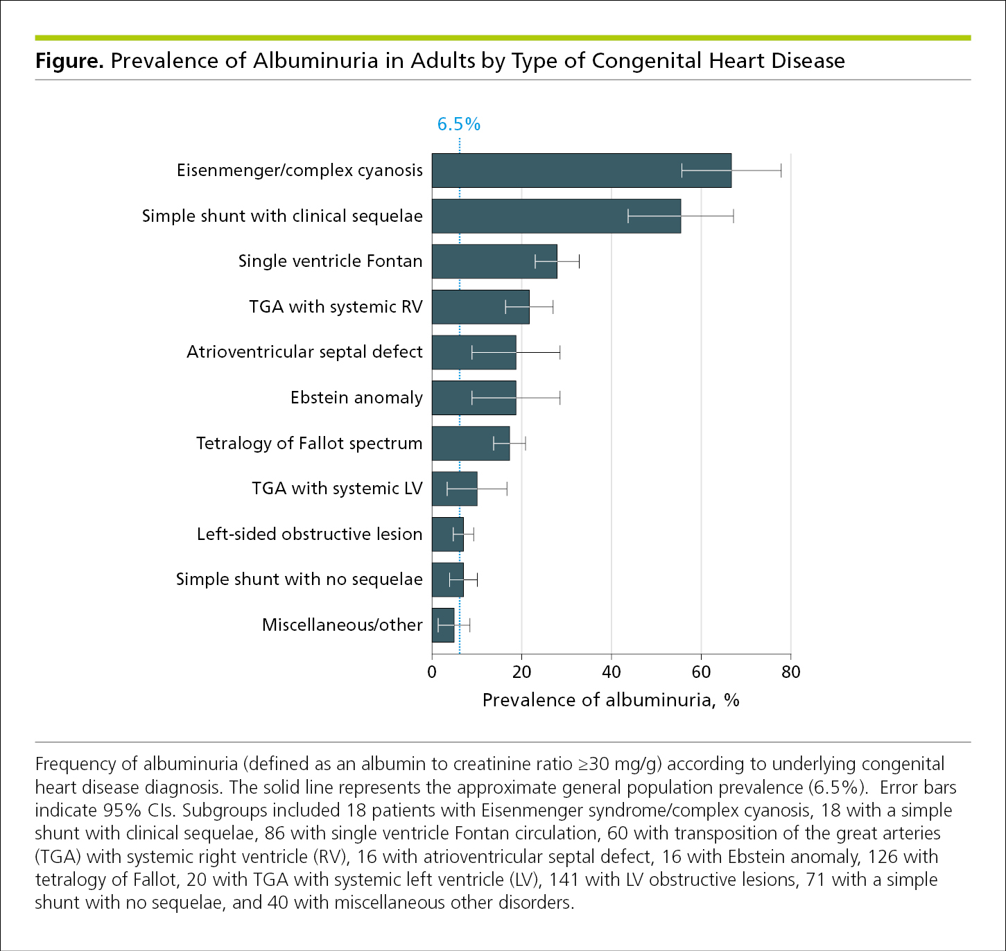
Bar graphs are used to display frequencies (counts or percentages) according to categories shown on a baseline or x-axis. Bar graphs also allow subcategories, making it easy to compare within and between categories. Bar graphs are less ideal for showing trends over time because readers must visually connect the tops of the bars.⁷ Bar graphs are not appropriate for representing summary statistics (eg, means with SDs or odds ratios with 95% CIs). A bar graph is often vertical, with frequencies shown on a vertical axis (Figure 4.2-7). A horizontal arrangement has advantages when the categories have long titles or when there are a large number of categories and there is insufficient space to fit all the columns required for a vertical bar chart (Figure 4.2-8). Data in each category are represented by a bar. Bars should have the same width, be separated by a space, and be wider than the space between them. Bar lengths are proportional to frequency, the scale on the frequency axis should begin at 0, and the axis should not be broken. All bars must have a common baseline to facilitate comparison.¹⁴

Categories of data should be presented in logical order and be consistent with other figures and tables in the article. The baseline of a bar graph is not a coordinate axis and therefore should not have tick marks. If the data plotted are percentages or rates, use error bars to show statistical variability (Figure 4.2-7). Because variability (error) is not always symmetrical around the values plotted, error bars should be plotted in both directions (not just above the values).¹ Note that in Figure 4.2-7 the bars are presented in the same order in each grouping and error bars show statistical variability (95% CIs).

Figure 4.2-7. Vertical Bar Graph With Shading to Distinguish the 3 Groups That Are Compared

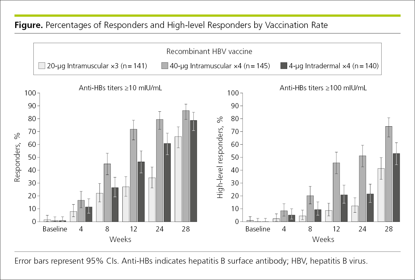
Figure 4.2-8. Horizontal Bar Graph With the Frequencies on the x-Axis and Categories Displayed Vertically

Bar graphs may be used to compare frequencies among groups. In most cases, the number of bars in a grouped bar graph should not exceed 3. Colors or tones used to designate each group should be distinct. To ensure that bars in black-and-white figures are distinguishable, a contrast in shading of at least 30% for adjacent bars is suggested. Color or shades of gray should be used instead of patterns and cross-hatching (eg, diagonal lines) on bars (Figure 4.2-7).

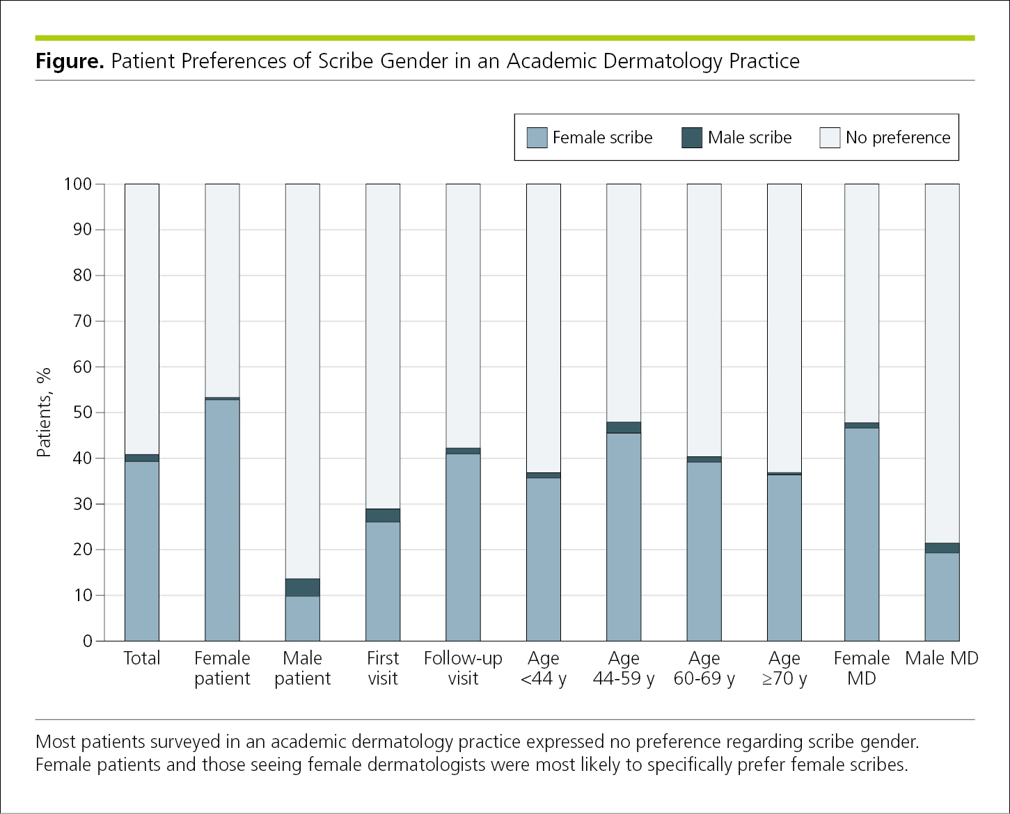
4.2.1.5.1 Component (Stacked) Bar Graph.

Component bar graphs (or divided or stacked bar graphs) display the proportion of components constituting the total group, represented by the whole bar (Figure 4.2-9). Individual components are designated by distinguishing formats, such as different shading. When possible, it is preferable to use clusters of individual bars to represent each component because the only values easily interpreted in a component bar graph are the total and the end segments,¹⁴ as is evident in Figure 4.2-9.

Figure 4.2-9. A Component Bar Graph

4.2.1.6 Pie Charts.

Pie charts should be avoided in scientific publications but are sometimes used in publications for lay audiences.¹⁵ Like the component bar graph, pie charts compare relationships among component parts. Categories are represented by sections, with the area of the section being proportional to the relative frequency of each category. The angular areas of the individual components of pie charts may be difficult to compare in series of pie charts. Usually, data depicted in pie charts can be summarized in the text or in a table.¹⁶

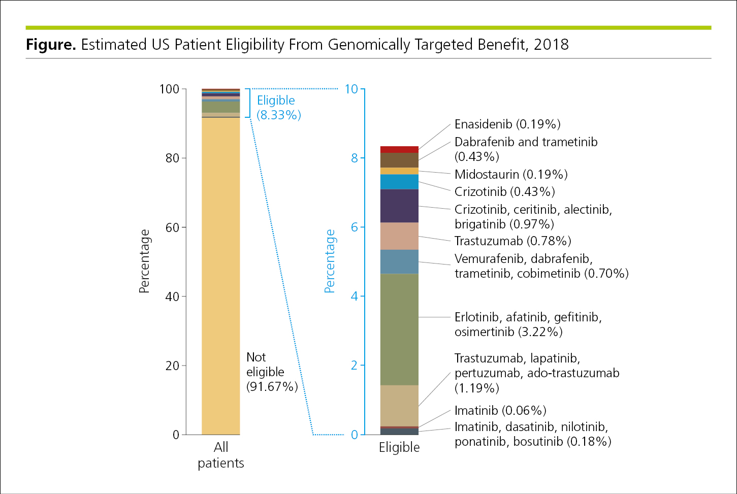
A more complex pie chart with large differences in the size of its divisions (Figure 4.2-10) can be reformatted as a bar graph in which the section encompassing the smaller divisions is enlarged in a second bar (Figure 4.2-11).

Figure 4.2-10. Example of a Complex Pie Chart

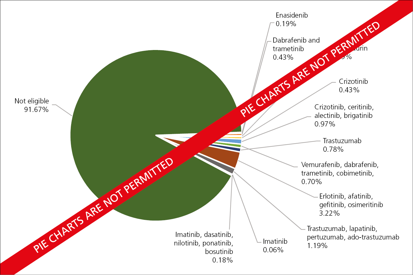
Figure 4.2-11. The Same Data in Figure 4.2-10 Reformatted as a Bar Graph

4.2.1.7 Dot (Point) Graphs.

Dot or point graphs display quantitative data other than counts or frequencies on a single scaled axis according to categories on a baseline (the scaled axis may be horizontal or vertical). Point estimates are represented by discrete data markers, preferably with error bars (in both directions) to designate variability (Figure 4.2-12).

Figure 4.2-12. A Dot Plot (Point Estimate Graph) Depicting Categorical Data

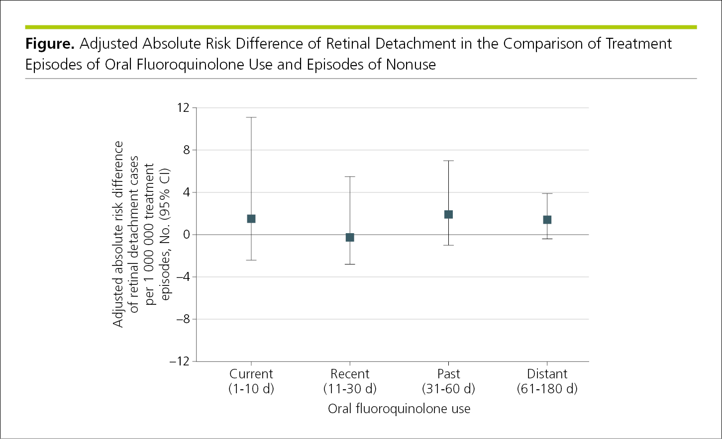
Note the use of a baseline at y = 0 in Figure 4.2-12 when values are both positive and negative, and error bars are drawn in both directions.

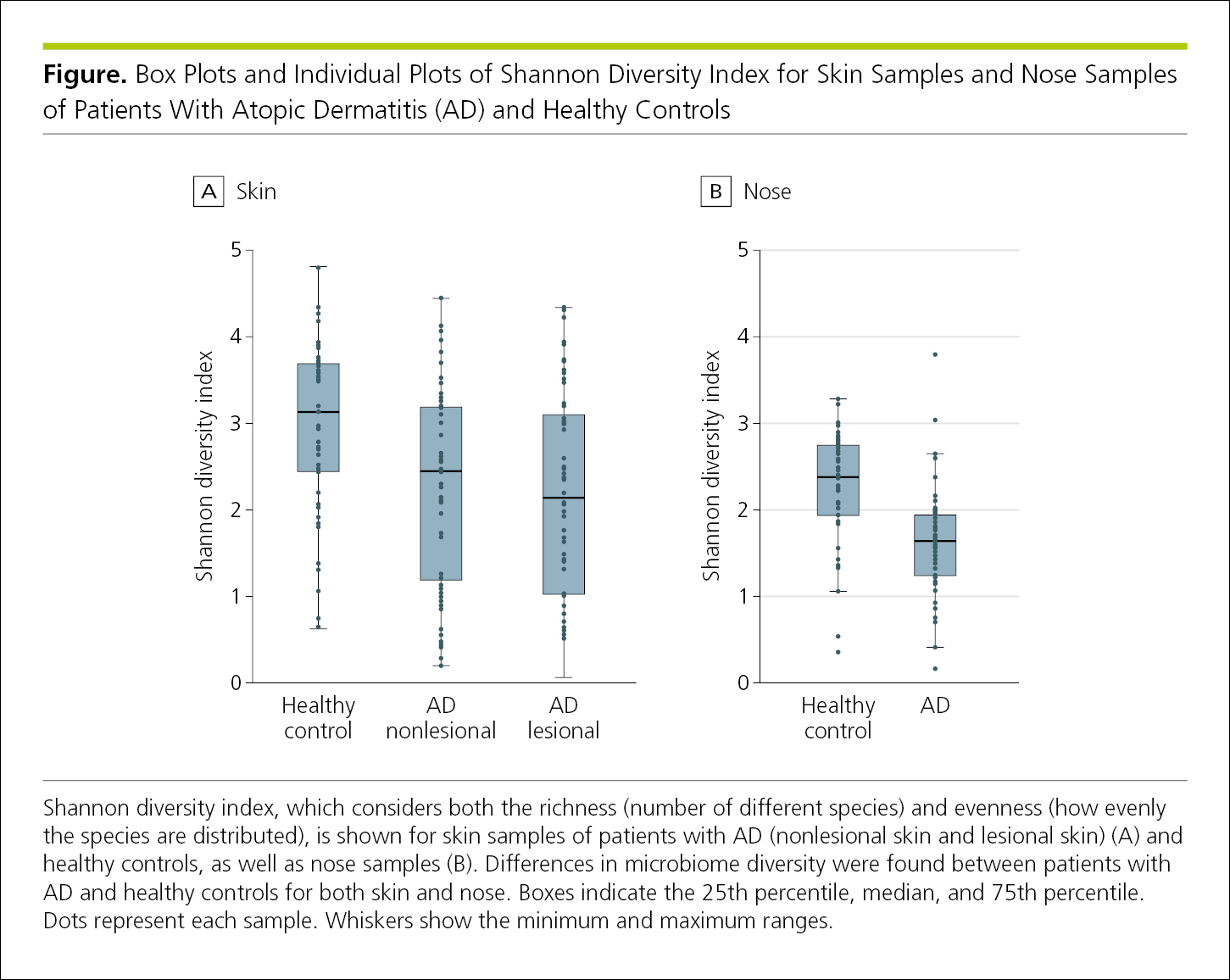
4.2.1.8 Box and Whisker Plots.

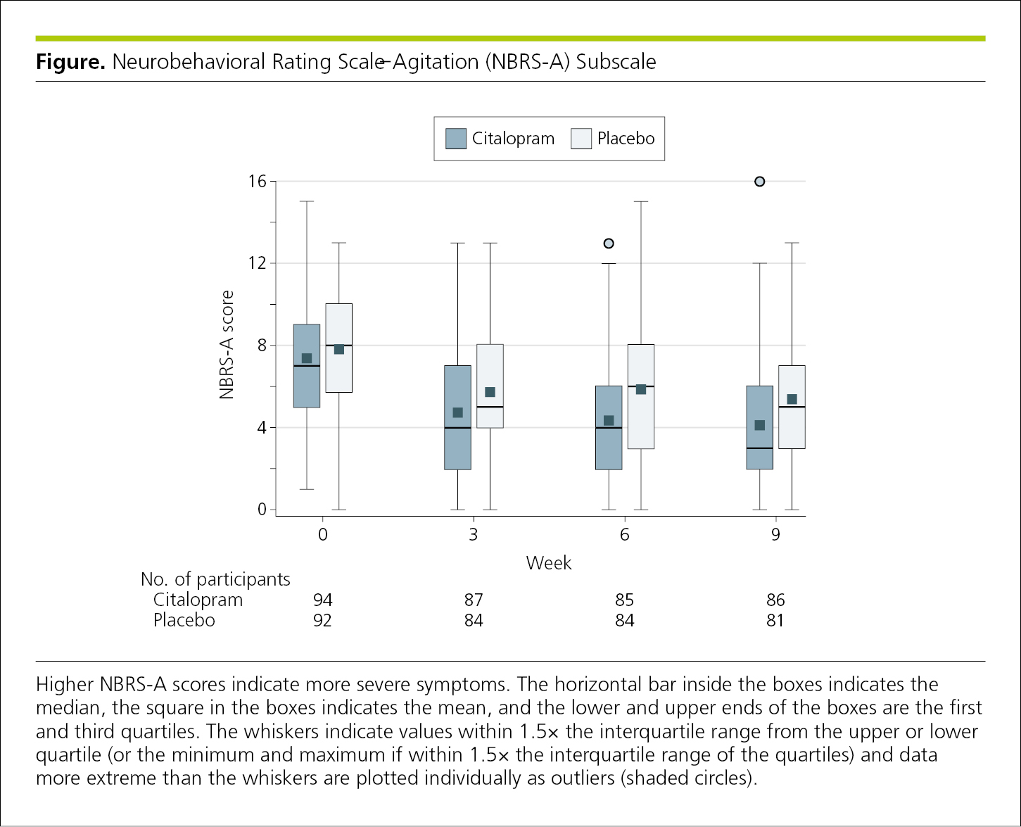
Box and whisker plots (also known as box plots) are useful for displaying data based on their quartiles. In general, summary data presentation is best reserved for larger sample sizes; there is little point in showing data from fewer than 10 contributing sources. Box and whisker plots can provide more information about a distribution than the typical bar graph while still emphasizing the values of interest¹ and can allow readers to better compare distributions. Typically, the ends of the “boxes” represent the 25th and 75th percentiles. Usually a horizontal line inside the box indicates the median or mean, and the “whiskers” represent the upper and lower adjacent values.¹ Outlier data are typically shown as circles plotted beyond the whiskers (Figure 4.2-13). What each element represents should be clearly indicated in the figure legend.

Figure 4.2-13. Box and Whisker Plot With Each Element Defined in the Legend

4.2.1.9 Individual-Value Plots.

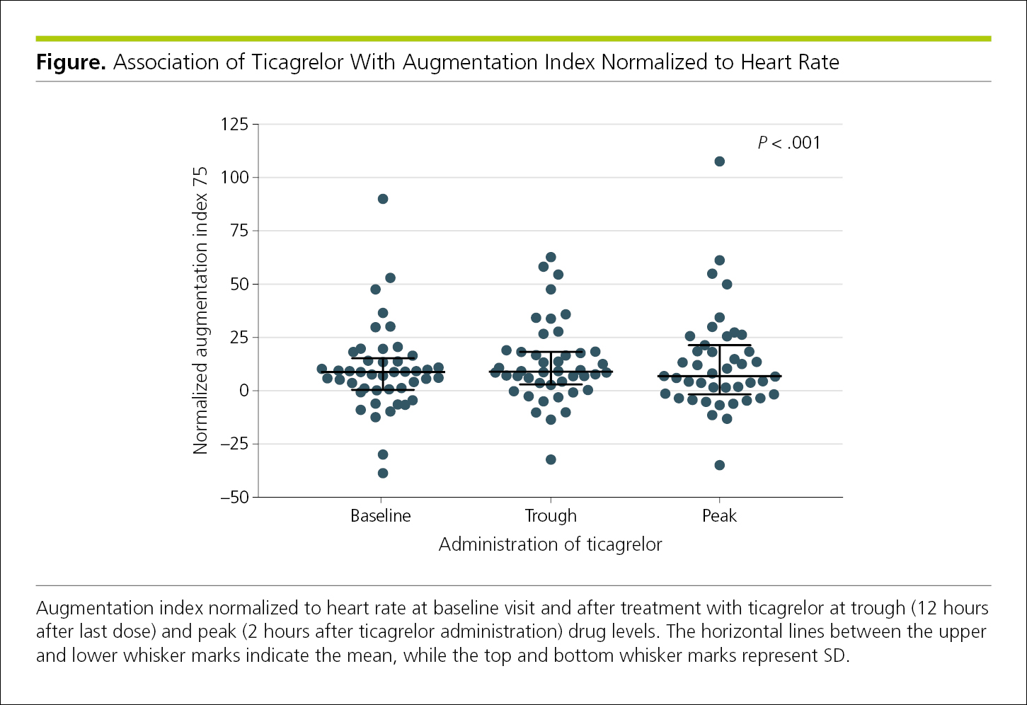
Individual values can be plotted on a graph to illustrate the full distribution of findings, for example, at different time points. The mean or median value for the group may be depicted by a horizontal line near the midpoint of the spread to illustrate the central tendency, and error bars may also be included to represent statistical variance (Figure 4.2-14). The horizontal lines between the upper and lower error bars in Figure 4.2-14 indicate the mean; the top and bottom error bars represent SDs.

Figure 4.2-14. Individual-Value Plot

4.2.1.10 Paired Data and Spaghetti Plots.

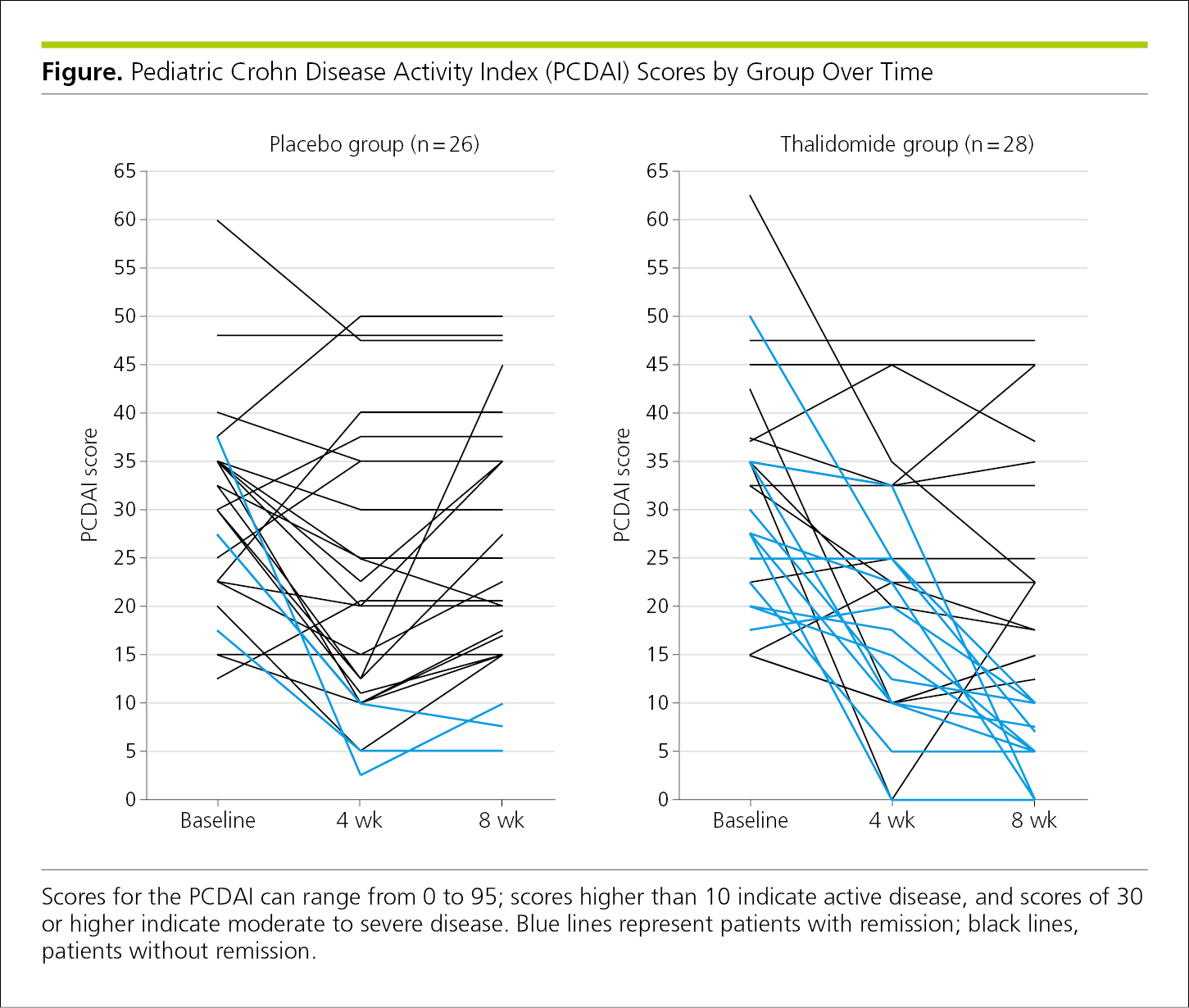
Paired data may be plotted from each study participant and compared. Data are typically plotted at baseline and at 1 or more prespecified outcome points (Figure 4.2-15). If several overlapping lines with 3 or more data points each are plotted together, these graphs are called spaghetti plots^17,18 or parallel coordinate line segment plots.¹⁹ These plots work better for a small number of study participants.¹⁹ However, although it can be difficult to distinguish the data for the individual lines, spaghetti plots can show trends over time.¹⁸ In Figure 4.2-15, the colored lines indicate another level of information (patients with remission are in blue).

Figure 4.2-15. Spaghetti Plots of Scores, by Group, for Patients at Baseline and 2 Specified Measurement Times

4.2.1.11 Forest Plots.

The results of meta-analyses and systematic reviews are often presented in summary figures known as forest plots.¹ Forest plots—the graphical display of individual study results and, usually, the weighted mean of studies included in a meta-analysis—are one way of summarizing the review’s results for a specific outcome.²⁰ In these figures, the estimated effects (and 95% CIs) are presented both tabularly and graphically (Figure 4.2-16). The first column typically lists the sources of the data, most often previously published studies along with their publication years and citations (which should appear in the reference list of the meta-analysis with links to the originals).²⁰ The sources should be listed in a meaningful order, such as by date or duration of follow-up. The plot portion allows readers to see the information from the individual studies at a glance. It provides a simple visual representation of the amount of variation among the results of the studies, as well as an estimate of the overall result of all the studies together.²¹ Various conventions are used in forest plots, including proportionally sized boxes to represent the weight of each study in the meta-analysis and the use of a diamond to show the overall effect at the bottom of the plot. It is important to include headers at the top of the plot to the left and right of the effect size or point estimate line (eg, 1.0 in Figure 4.2-16) to indicate which variables, interventions, exposures, or outcomes are favored. Note that the values plotted are also provided in the hazard ratio (HR) column. The dotted line at 1.0 represents no effect and allows for quick visualization of the effect of each study listed. The overall I ² and P values are provided in the figure.

Figure 4.2-16. Effect Sizes and Pooled (Combined) Data in a Meta-analysis, With the Size of the Data Markers Sometimes Indicating the Relative Weight of Each Study, Depending on the Software Used to Generate the Figure

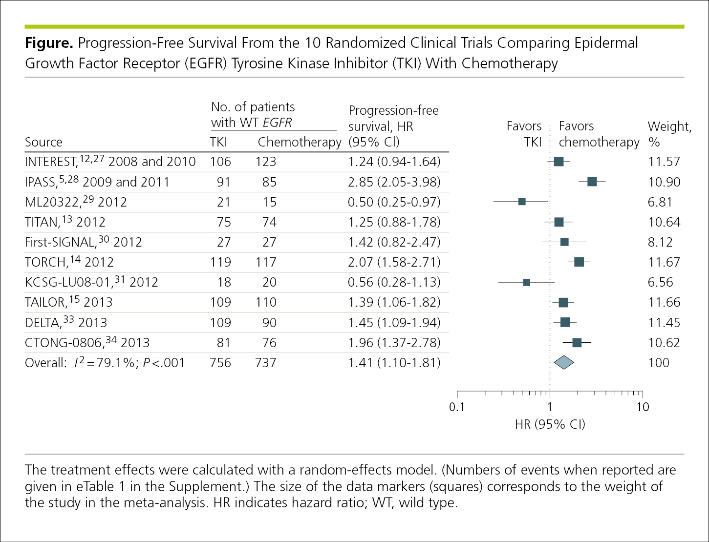
In most cases, forest plots should be plotted on a log scale. Log scales are useful for presenting rates of change and are presented such that 2 equal distances represent the same percentage change.¹ For example, the distance on the x-axis between the ticks labeled 1 and 2 would be the same length as between the ticks labeled 2 and 4. Log scales begin at 1 (or a proportion thereof), not 0, and do not plot negative values (Figure 4.2-16).¹

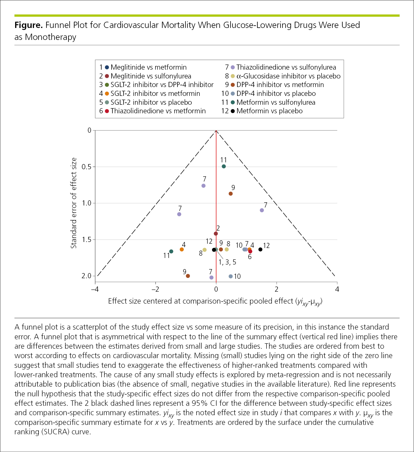
4.2.1.12 Funnel Plots.

A funnel plot is a scatterplot of the effect size for each of the studies used in a meta-analysis vs some measure of the effect size’s precision²² and may be useful to assess the validity of the meta-analysis.²³ In the absence of bias, the plot will resemble a symmetrical inverted funnel (Figure 4.2-17). Conversely, if bias exists, funnel plots will often be skewed and asymmetrical.

Figure 4.2-17. Funnel Plot Used to Detect Bias in a Meta-analysis

4.2.1.13 Hybrid Graphs.

Occasionally, a combination of 2 graphing techniques can provide more information than either technique alone (Figure 4.2-18). This figure shows the full distribution of values and also allows readers to better compare those distributions.

Figure 4.2-18. Individual-Value Plots Overlaid With Box Plots

4.2.2 Diagrams.

4.2.2.1 Flowcharts.

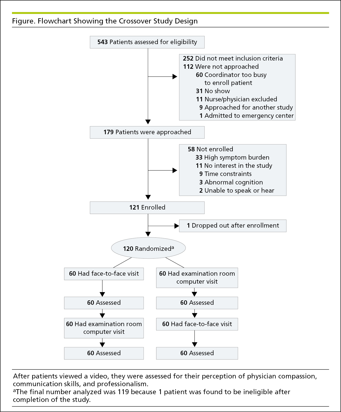
Flowcharts show the sequence of activities, processes, events, operations, or organization of a complex procedure or an interrelated system of components and sometimes function as visual summaries of a study. Flowcharts are useful to depict study protocol or interventions, to demonstrate participant recruitment and follow-up such as in a randomized clinical trial (CONSORT [Consolidated Standards of Reporting Trials])²⁴ (Figure 4.2-19, and Figure 19.2-1 in 19.0, Study Design and Statistics), or to show inclusions and exclusions of samples in other types of studies, such as in systematic reviews and meta-analyses (PRISMA [Preferred Reporting Items for Systematic Reviews and Meta-analyses])²⁴ (Figure 4.2-20) and studies of diagnostic accuracy (STARD [Standards for the Reporting of Diagnostic Accuracy Studies]).²⁴ When the assignment in an unrandomized clinical trial was not random (eg, if the treatment was allocated or assigned), a rectangle is used instead of an oval (Figure 4.2-21). A crossover study involves 2 or more interventions. In it, all of the study participants receive all the interventions, but those interventions are assigned in a random order²⁵ (Figure 4.2-22).

Figure 4.2-19. Flowchart for a Randomized Clinical Trial Using CONSORT Criteria

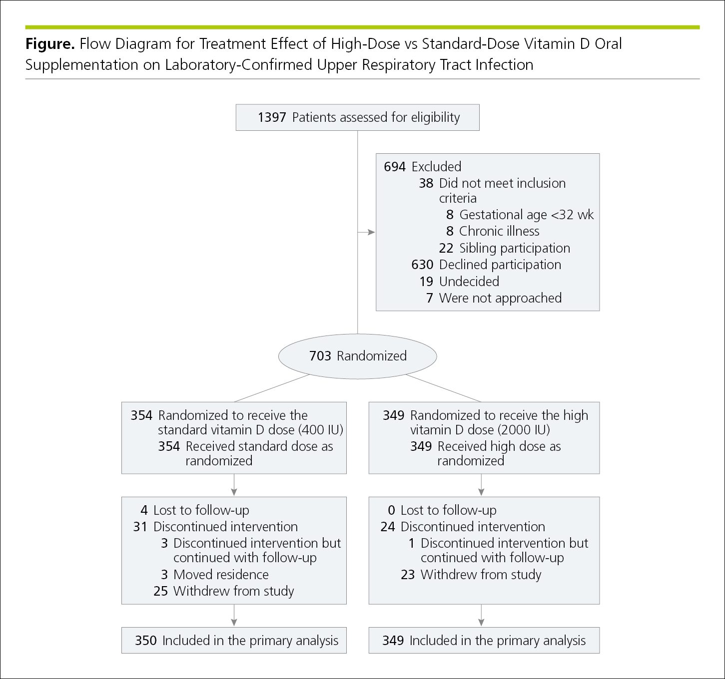
In the JAMA Network journals, the randomization point is the only oval; all other entries are rectangular. Note that the allocation point in a nonrandomized trial uses a rectangular box rather than an oval to distinguish it from a flowchart for a randomized clinical trial (Figure 4.2-21).

Figure 4.2-20. Flowchart for a Systematic Review and Meta-analysis Using PRISMA Criteria²⁴

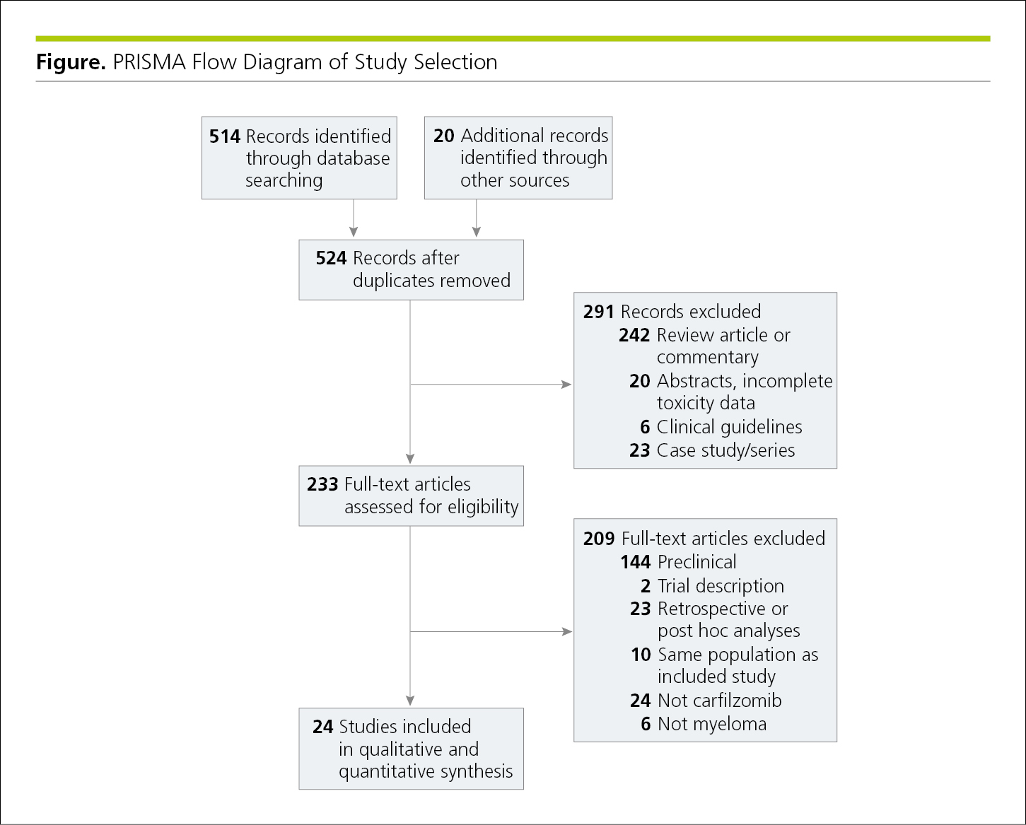
Figure 4.2-21. Flowchart for a Clinical Trial in Which Assignment Was Allocated

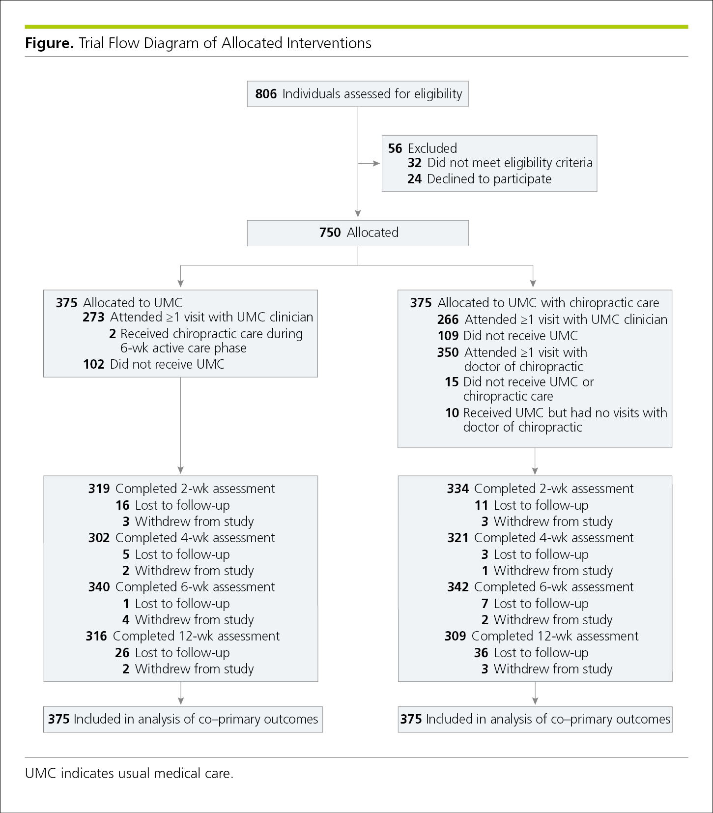
Figure 4.2-22. Flowchart for a 2-Arm Crossover Study

4.2.2.2 Decision Trees.

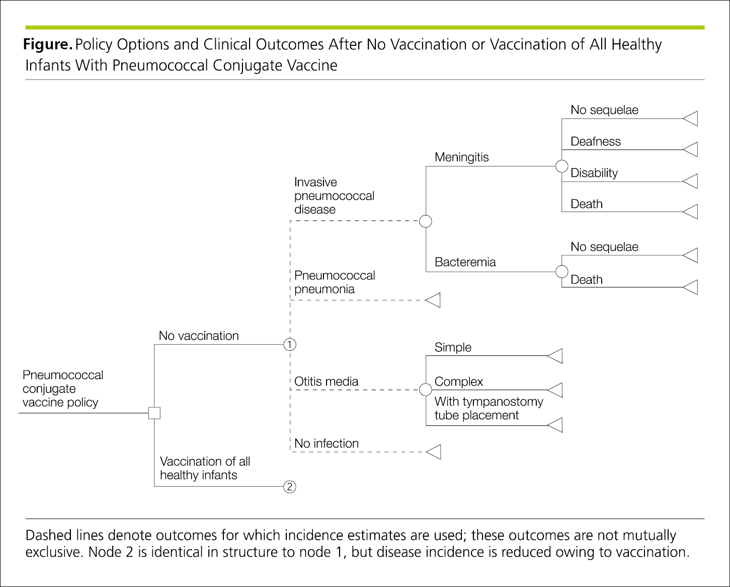
Decision trees are analytical tools used in cost-effectiveness and decision analyses.²⁶ The decision tree displays the logical and temporal sequence in clinical decision-making and usually progresses from left to right (Figure 4.2-23). A decision node is a point in the decision tree at which several alternatives can be selected and, by convention, is designated by a square. A chance node (probability node) is a point in the decision tree at which several events, determined by chance, may occur and, by convention, is designated by a circle.

Figure 4.2-23. Decision Tree Showing Options and Possible Outcomes From Left to Right

4.2.2.3 Algorithms.

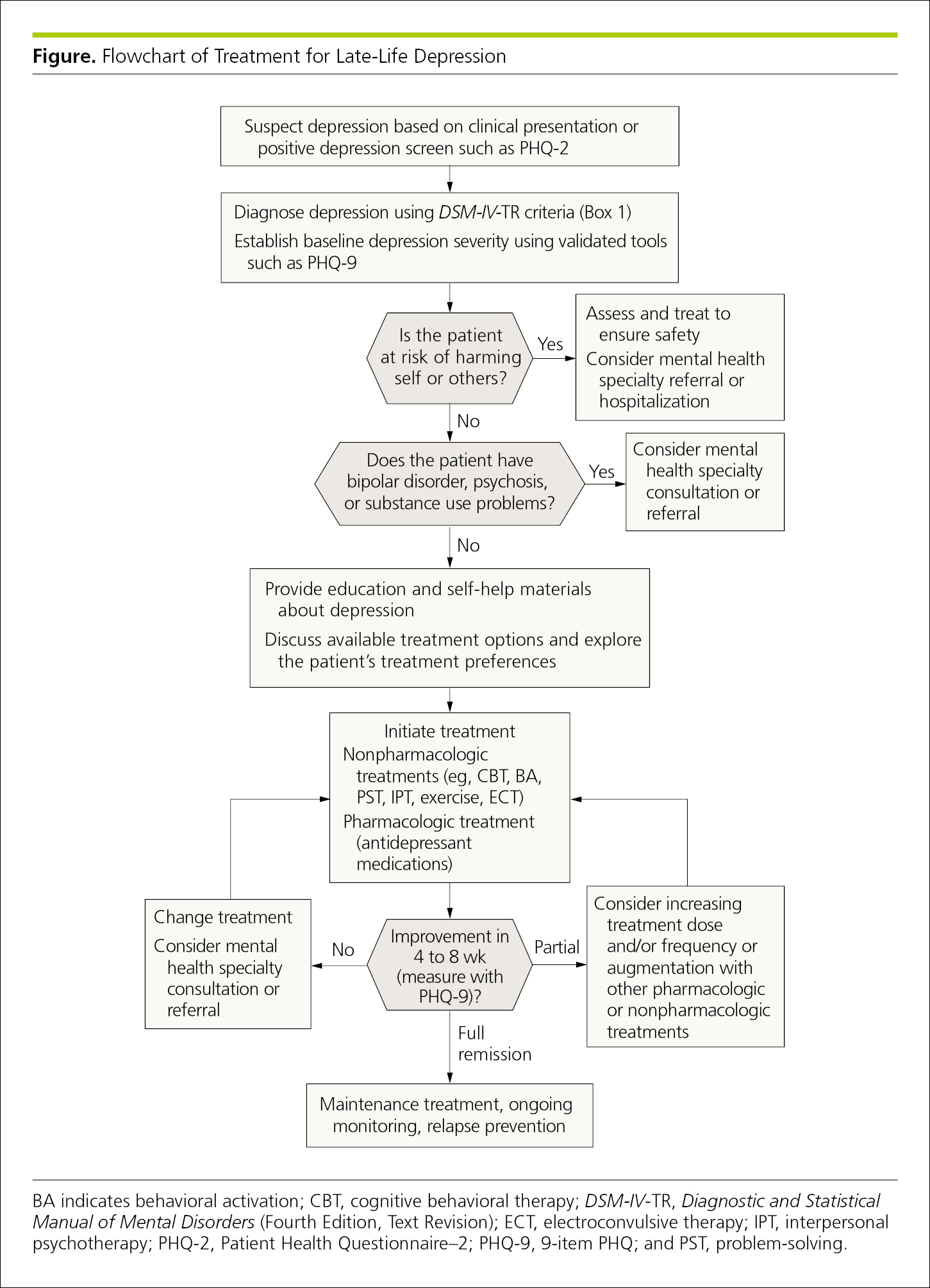
Algorithms contain branched pathways to permit the application of carefully defined criteria in the task of identification or classification,²⁷ such as to aid in clinical diagnosis or treatment decisions. Standard box shapes are used to indicate various steps in the algorithm. For example, a diamond or hexagon indicates a decision box, which has at least 2 arrows leading to different paths in the algorithm. A rectangle or square indicates an action or decision box. Algorithms use arrows to guide readers through the process, and yes and no are marked directly on the pathways (Figure 4.2-24).

Figure 4.2-24. Treatment Algorithm

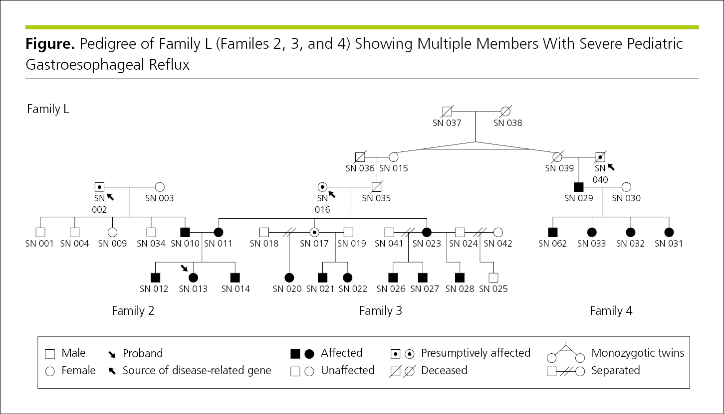
4.2.2.4 Pedigrees.

Pedigrees illustrate familial relationships and are often used in the study and description of inherited disorders. Standard symbols are used to indicate each person’s sex, vital status (living or dead), and whether he or she has the condition or genetic component in question, if known. Symbol shapes and lines drawn horizontally and vertically between the symbols convey information about the generations depicted and relationships among individuals,²⁸ with the earliest generation at the top of the figure (Figure 4.2-25) (see 14.6.6, Pedigrees). If the sex of each person is not relevant to the discussion and there may be a concern about identifiability or confidentiality, diamonds or other sex-neutral symbols can be substituted for the standard circles and squares (see 5.8.3, Protecting Research Participants’ and Patients’ Rights in Scientific Publication, Rights in Published Reports of Genetic Studies). A key inside the figure plot explains each symbol.

Figure 4.2-25. Hypothetical Pedigree of Multiple Generations in 3 Related Families, With the Probands Indicated by an Arrow

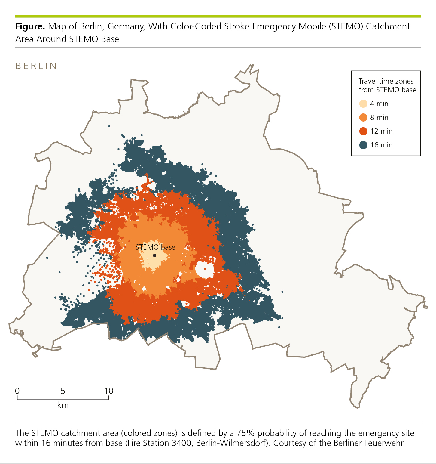
4.2.3 Maps.

Maps are useful to demonstrate relationships or trends that involve location and distance or to illustrate study sampling methods (Figure 4.2-26). Maps may be used to demonstrate geographic relationships (eg, spread of a disease). Choropleth maps depict quantitative data (eg, relative frequencies by county, state, country, continent, province, or region), with differences in numerical data, such as rates, shown by shading or colors. Authors should verify map details to avoid misspelled or incorrect names, deleted features, distorted geographic relationships, misplaced or missing cities, and misplaced boundaries.

Figure 4.2-26. Map to Show the Distribution by Distance of Travel Time (via Ambulance) to the Treatment Site

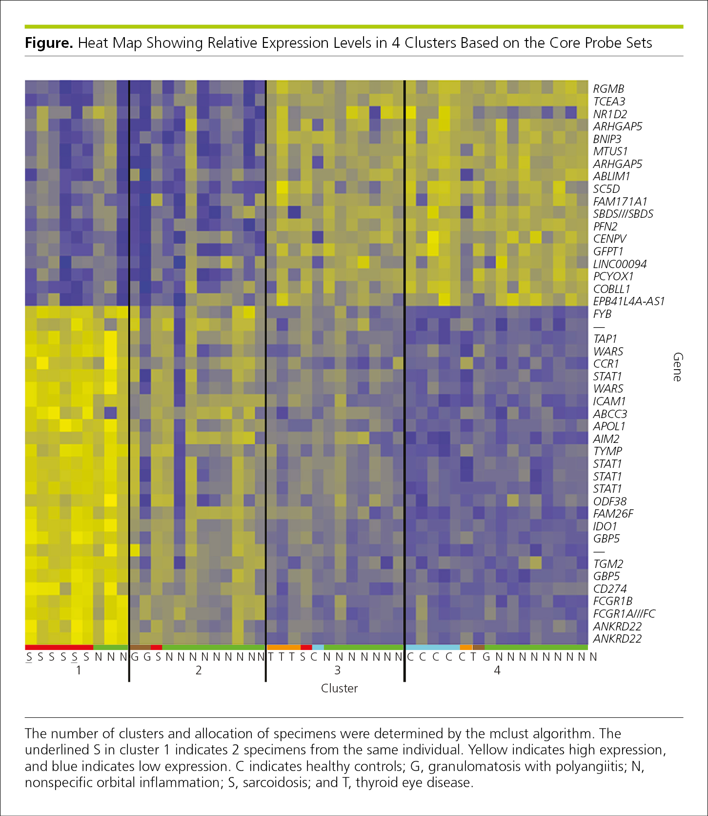
A heat map is a graphical representation of data that simultaneously reveals row and column hierarchical cluster structure in a data matrix.^29,30 It consists of rectangular tiling, with each tile shaded on a color scale to represent the value of the corresponding element of the data matrix. Heat maps are commonly used to display gene expression (Figure 4.2-27). Each row in the grid represents a gene and each column a sample. The color and intensity of the boxes are used to represent changes (not absolute values) of gene expression.³¹ The heat map may also be combined with clustering methods that group genes and/or samples based on the similarity of their gene expression pattern, with similar rows and columns near each other.^29,30 Such grouping can be useful for identifying genes that are commonly regulated or biological signatures associated with a particular condition (eg, a disease or an environmental condition).³¹

Figure 4.2-27. Genetic Heat Map Showing Relative Expression Levels in 4 Clusters (Groups of Samples That Are More Closely Related to One Another³⁰) Based on the Core Probe Sets

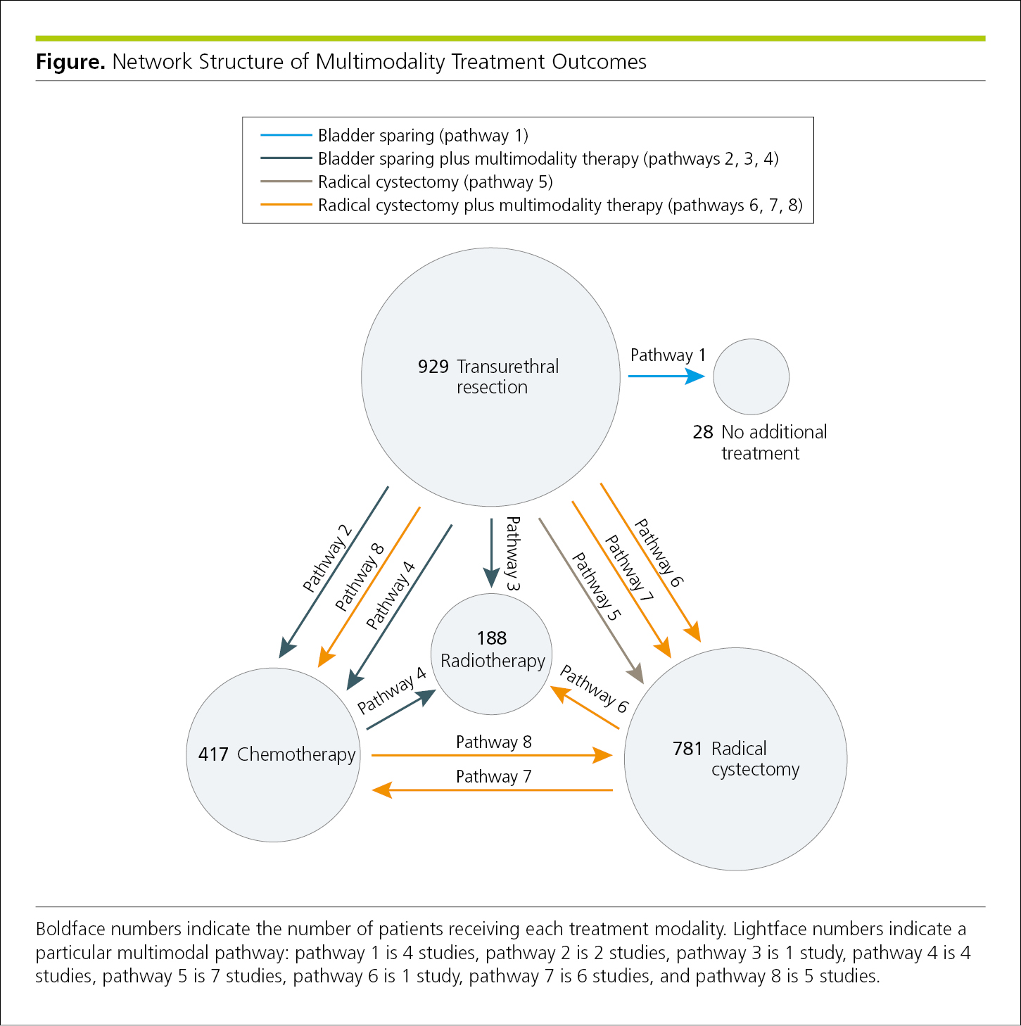
Network maps, visual representations of the physical connectivity among separate points in a network,³² can illustrate movement (Figure 4.2-28) or other relationships among groups or outcomes (Figure 4.2-29).

Figure 4.2-28. A Network Map Shows Movement From the Point of Diagnosis to Different Areas of a Hospital by 1152 Patients With Clostridioides difficile (formerly Clostridium difficile) Infection Who Were Diagnosed in the Emergency Department During a Single Year

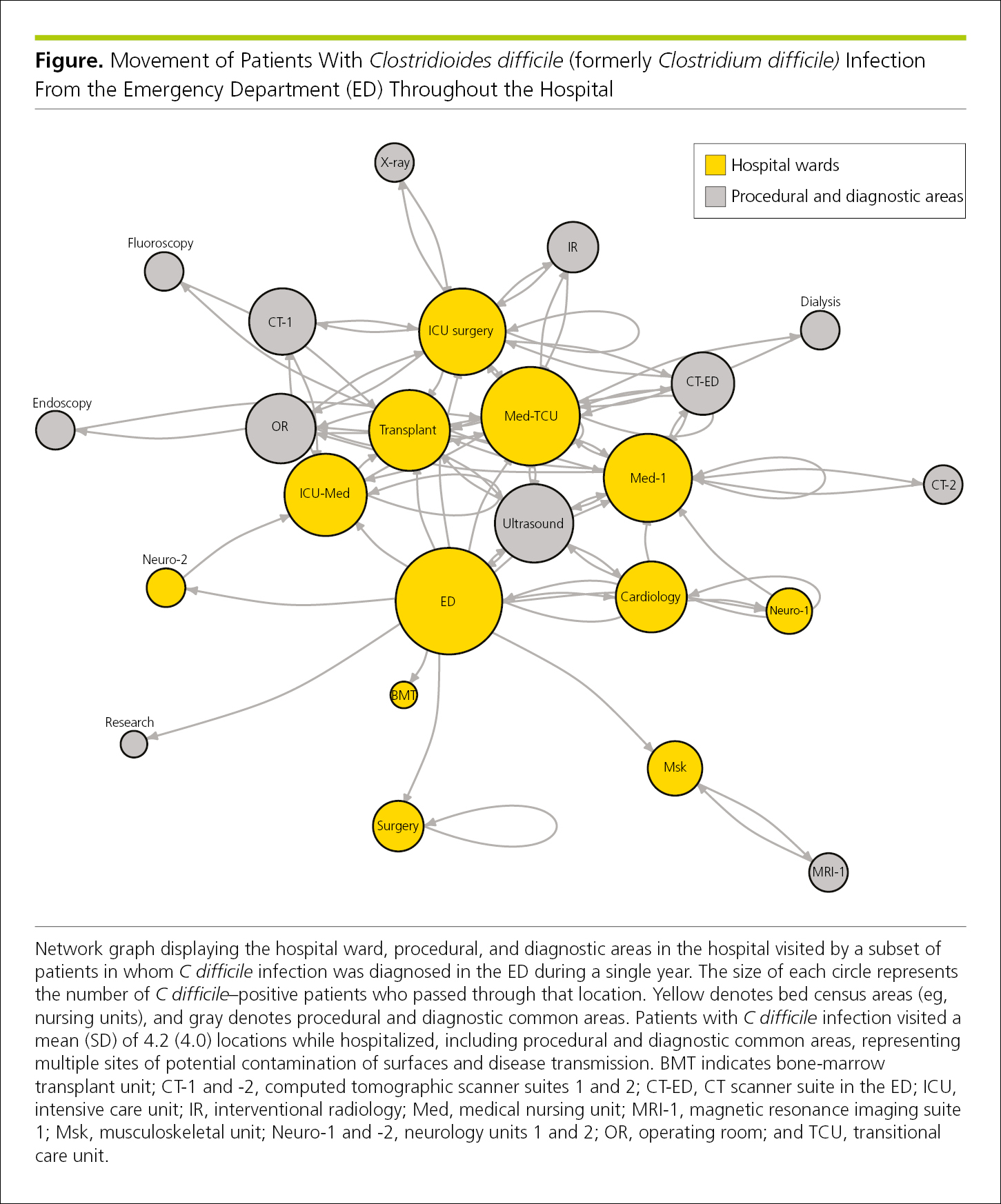
Figure 4.2-29. Network Map Illustrating Treatment Outcomes for Multiple Treatment Modalities

4.2.4 Illustrations.

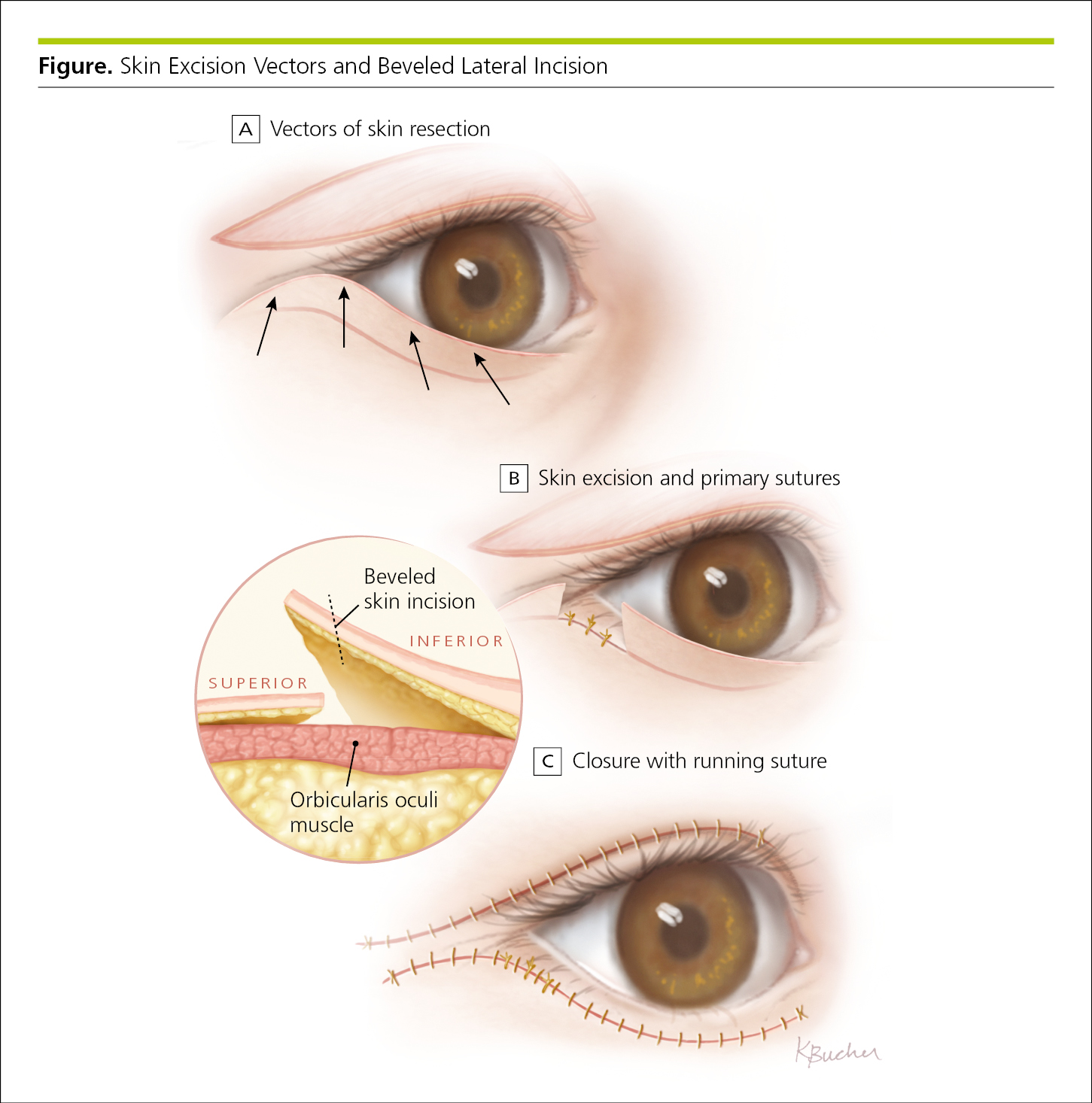
Illustrations may explain physiologic mechanisms, describe clinical maneuvers and surgical techniques, and provide orientation to medical imaging. Complex interactions often are easier to convey and understand in an illustration than in text or tables (Figure 4.2-30).

Figure 4.2-30. Illustration Depicting Anatomy and Surgical Techniques

4.2.5 Photographs and Clinical Imaging.

Photographs and other images in biomedical articles are used to display clinical findings, experimental results, or clinical procedures. Such figures include radiographs (Figure 4.2-31) and those from other types of medical imaging (Figure 4.2-32 and Figure 4.2-33), photomicrographs (Figure 4.2-34), and photographs of patients (Figure 4.2-35) and biopsy specimens (Figure 4.2-31). If an individual can be identified in a photograph, the author should obtain a signed statement granting permission to publish the photograph from the identifiable person (see 4.2.11, Consent for Identifiable Patients, and 5.8.2, Patients’ Rights to Privacy and Anonymity and Consent for Identifiable Publication).

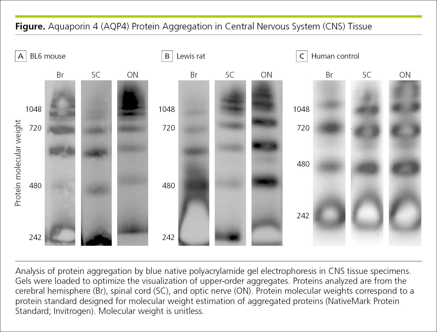
The availability of digital imaging allows for enhancement of images of photographic scientific data, such as clinical images (Figure 4.2-33) or gel electrophoresis bands (Figure 4.2-36).³³ Such digital manipulation may produce misleading or fraudulent images (see 5.4.1, Scientific Misconduct, Misrepresentation: Fabrication, Falsification, and Omission). Some publications require that authors submit the original images; others ask authors to list image adjustments in the paper itself.^33,34

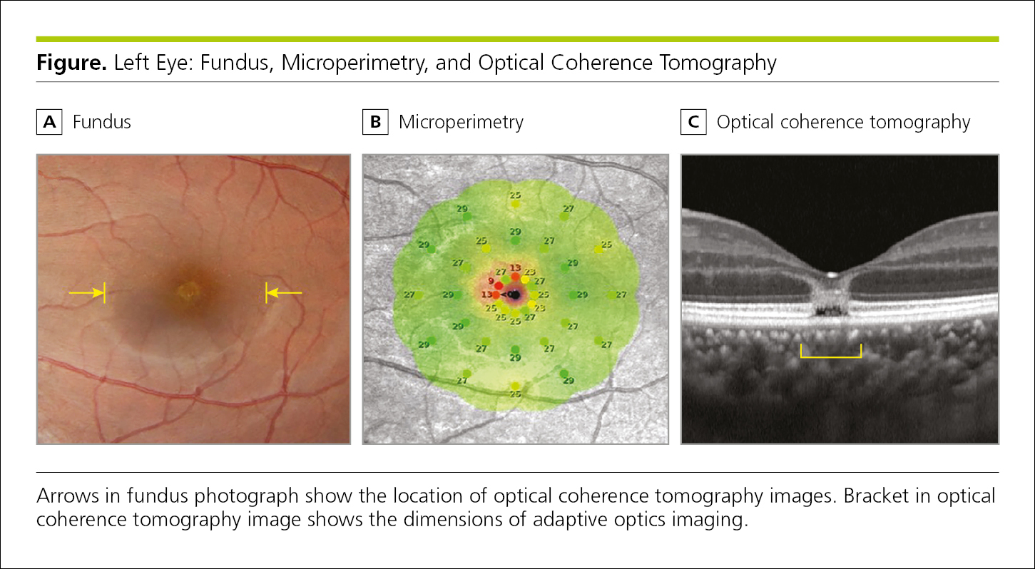
When a figure includes labels, arrows, or other markers to identify or point out certain features, these should be explained in the figure legend (Figure 4.2-32).

Figure 4.2-31. Radiographs Showing 2 Views of a Patient’s Left Femur Alongside an Immunohistochemically Stained Biopsy Specimen

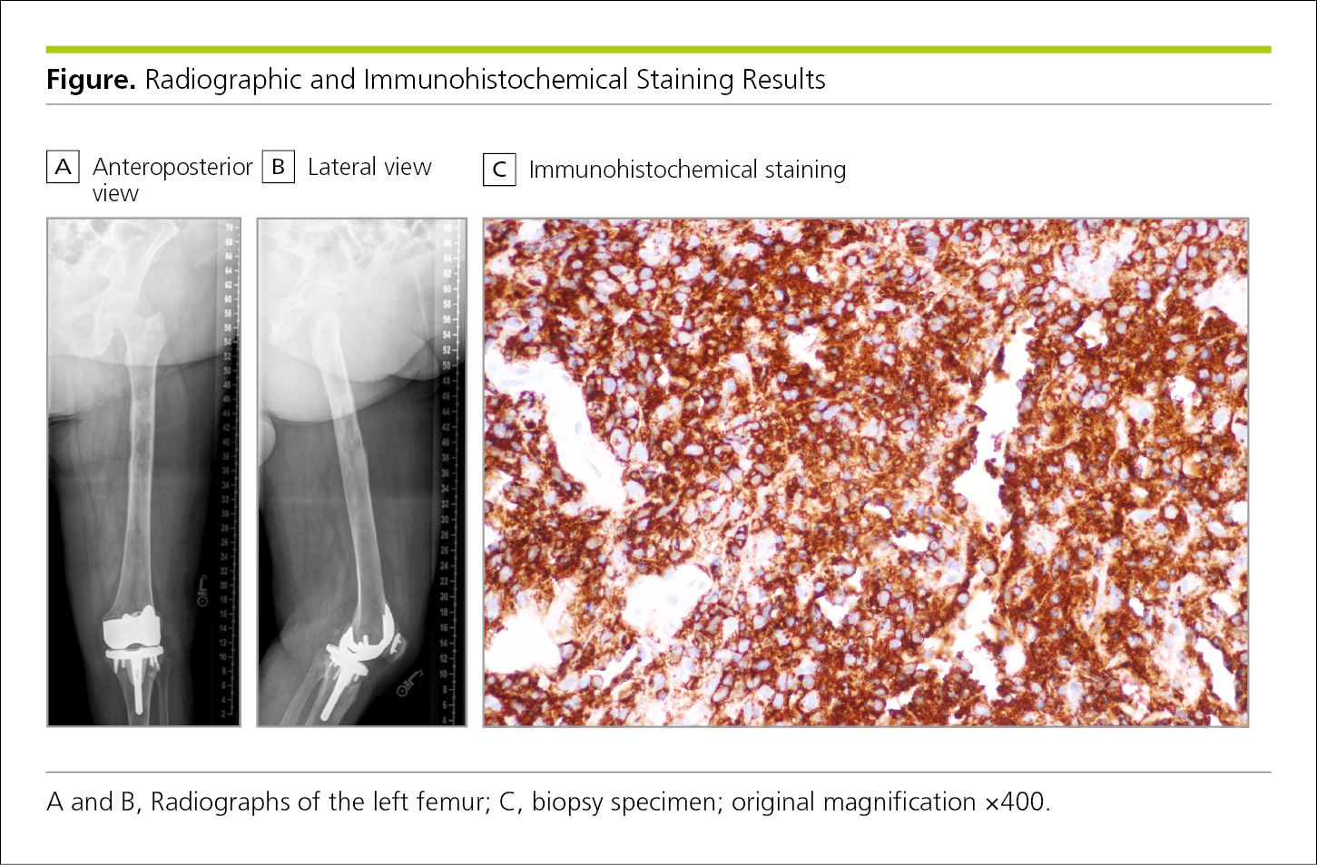
Figure 4.2-32. A Series of Magnetic Resonance Images Captured at Different Times Can Show Structural Changes Resulting From Disease or Treatment

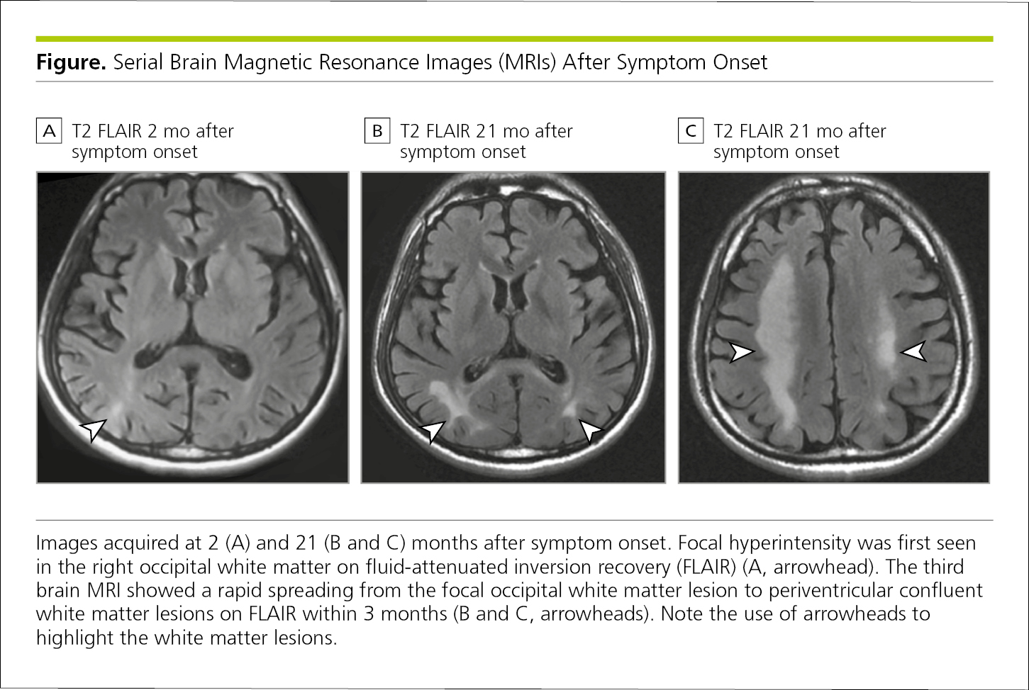
Figure 4.2-33. Clinical and Ultrasonographic Images of Brachial Artery Pseudoaneurysm Originating From the Profunda Brachii Artery

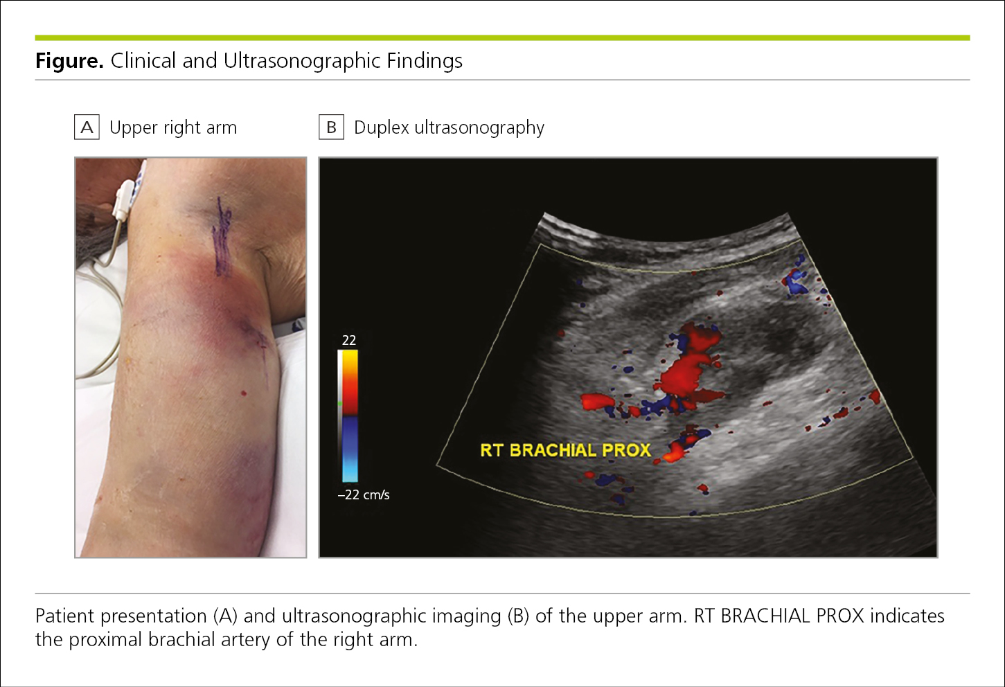
Figure 4.2-34. Photomicrograph of a Biopsy Specimen Illustrates the Use of Laser-Assisted Mass Spectrometry to Confirm Deposition of Gadolinium in Sclerotic Bodies of Gadolinium-Associated Plaques

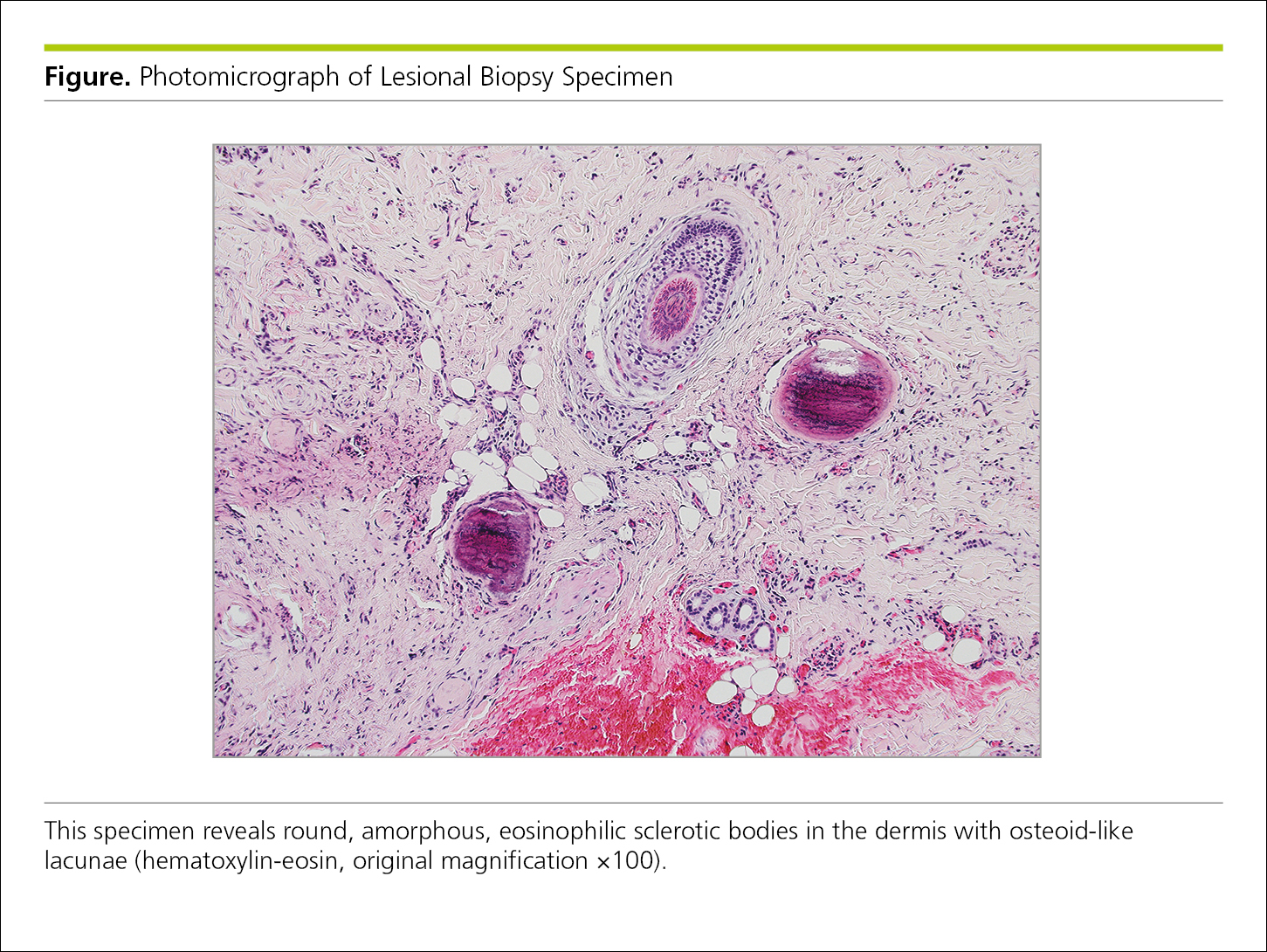
Figure 4.2-35. Photographs Showing Nasal Size Distortion in a Short-Distance Photograph Above a Diagram Illustrating How the Extent of Distortion Is Calculated

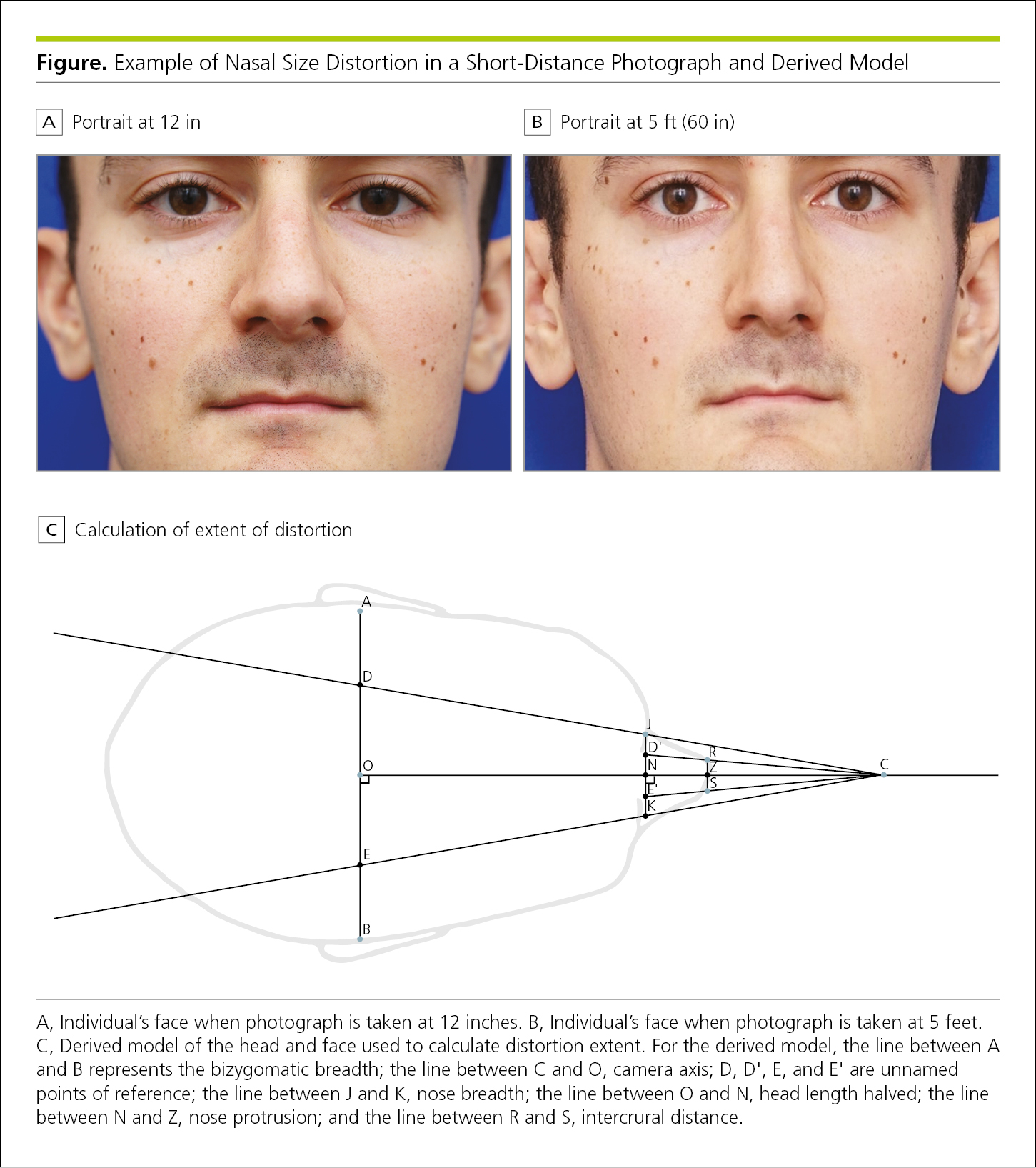
Figure 4.2-36. Gel Electrophoresis Shows Protein Aggregation in Central Nervous System Tissue From a BL6 Mouse (A), a Rat (B), and a Human (C)

4.2.6 Components of Figures.

Clear display of data or information is the most important aspect of any figure. For figures that display quantitative information, data values may be represented by dots, lines, curves, area, length, or shading based on the type of graph used.

4.2.6.1 Scales for Graphs.

The horizontal scale (x-axis) and the vertical scale (y-axis) indicate the values of the data plotted in a graph. In most graphs, values increase from left to right (on the x-axis) and from bottom to top (on the y-axis). Rarely, a third scale (secondary y-axis) may be relevant, also with values increasing from bottom to top (Figure 4.2-2). Data lines should be thicker than the scale lines to draw attention to the data.¹

4.2.6.1.1 Range of Values.

The range of values on the axes should be slightly greater than the range of values being plotted, so that the entire data set can appear within the area defined by the axes and most of the possible range of values on the axes will be used. Ideally, the range should include 0 on both axes, if 0 is a possible value for the variable being plotted. In line graphs, if a large range of values is necessary but cannot be depicted with a continuous scale in a single plot, the data may be broken into separate, smaller plots or an enlarged portion of the graph may be depicted in an inset (Figure 4.2-37). For single-axis plots, data that exceed the limits of the axes can be indicated with an arrowhead (such as in a forest plot).

Figure 4.2-37. Data With Widely Ranging Values

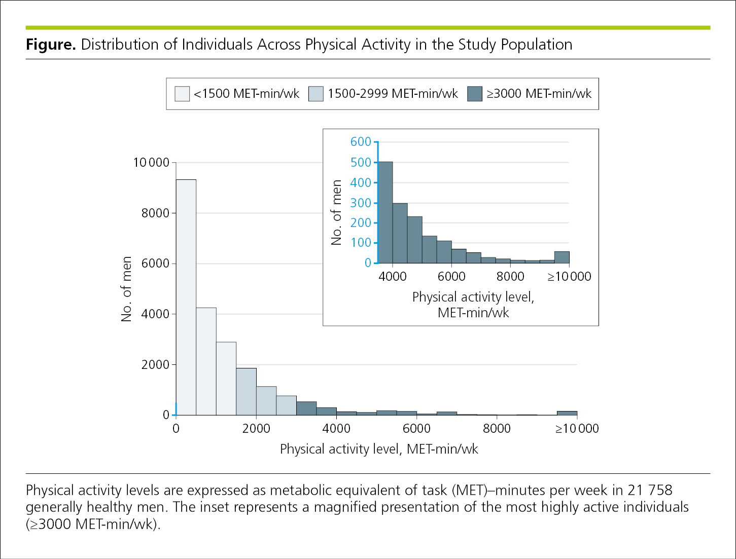
Note the use of blue on the y-axes of Figure 4.2-37 to show the relationship of the range of values between the plots.

4.2.6.1.2 Axis Scales.

Divisions of the scales on the graph axes should be indicated by intervals chosen to be appropriate, simple multiples of the quantity plotted, such as multiples of 2, 5, or 10.³⁵ Numbers that represent the values on the axis scale are centered on their respective tick marks. For linear scales, the axis must appear linear, with equal intervals and equal spacing between tick marks. However, logarithmic scales may be useful to show proportional rates of change (Figure 4.2-16) and to emphasize the change rate rather than the absolute amount of change when absolute values or baseline values for data series vary greatly. Tick marks and scale numbers should be placed outside the data field, just left of the y-axis and just below the x-axis, and centered on their respective tick marks. For numbers less than 1, include the digit zero before the decimal.⁴

4.2.6.2 Axis Labels.

Axes should be labeled with the type of data plotted and the unit of measure used. Data may represent numerical values, percentages, or rates. For numerical data, customary units of measure and their respective abbreviations or symbols should be used (see 13.12, Units of Measure). In single-axis graphs, categories should be clearly labeled along the baseline (Figure 4.2-9).

Axis labels should follow sentence-style capitalization, in consistency with other areas of the figure (such as in the figure key or direct labeling of lines). Phrases that appear on axes are generally easier to read in sentence style than when all major words are capitalized.

4.2.6.2.1 Symbols, Patterns, Colors, and Shading.

Symbols, line styles, colors, and shading characteristics used in the figure must be explained, preferably by direct labeling of components in the figure or, if infeasible, in a key. Alternatively, this information may be included in the legend. For a series of figures within an article, the types of symbols, line styles, colors, and shading should be used consistently. For example, if data for the intervention group and for the control group are designated as a heavy line and as a lighter line, respectively, then these same line styles should be used for similar data for these groups in subsequent figures. When lines cross or nearly do, line styles should be applied to ensure that they are easy to discriminate.

When data points are plotted, symbols should be distinguished easily by shape and color or shade. For example, if 2 symbols are needed, the recommended symbols are ○ and ●,³⁵ although □ and ■ or △ and ▲ may be used. A combination of these symbols can be used when 3 or more symbols are required. The shading or color of the symbols can designate specific data. For instance, in all figures in an article, ○ may indicate data for the placebo group and ● for the intervention group. A key to the different symbols can appear in the figure. In line graphs with connected data points, the curves should be labeled directly if there is room. Colors can be used to accentuate or deemphasize data groups.

In bar charts and other figures (such as maps), shading is preferable to cross-hatching and other patterns to distinguish groups. Patterns can be difficult to read both in print and online. Shades should be of appropriate gradations to show contrast (eg, 10%, 40%, and 70% black).

4.2.6.3 Error Bars.

For plotted data, error bars (depicting SD, SE, range, interquartile range, or CIs) are an efficient way to display variability in the data.³⁶ Error bars should be drawn to encompass the entire range of variability, not in just one direction (Figure 4.2-7) unless the prespecified analysis plan called for 1-sided hypothesis testing. Error bars should always be defined, either in the legend or on the plot itself.

4.2.6.4 Three-Dimensional Figures.

In most cases, figures should not be presented in 3-dimensional format. A 3-dimensional presentation is inappropriate for any figures that contain only 2 dimensions of data. Many software programs allow users to add enhancing elements to figures, but 3-dimensional display may confuse readers or distract from important graphical relationships. For instance, it may be difficult to read from the bar to the correct value on the axis. Most 3-dimensional presentations can be replotted into more straightforward graphics.

4.2.7 Titles, Legends, and Labels.

Many journals, including the JAMA Network journals, use separate titles and legends (also known as captions) to describe and clarify figures. Others combine the title and legend underneath the figure.

4.2.7.1 Titles.

The figure title follows the designation “Figure” numbered consecutively (ie, Figure 1, Figure 2) and does not appear in the figure itself. Articles that contain a single figure use the designator “Figure” (not “Figure 1”). The title is a succinct clause or phrase (perhaps 10-15 words) that identifies the specific topic of the figure or describes what the data show. In the JAMA Network journals, each major word in a figure title is capitalized and follows the same rules as for article titles (see 10.2, Titles and Headings). Some publications print the figure title above the figure and others place it under the figure, in sentence style.

Titles of figures, including diagrams, photographs, and line drawings, generally should not begin with a phrase identifying the type of figure:

However, a description of the type of figure may be required in certain circumstances to provide context and avoid confusion.

Figure 3. Fluorescein Angiogram Showing Widespread Retinal Capillary Nonperfusion and Marked Optic Nerve Head Leakage

Figure 4. Autoradiograph Demonstrating Loss of Heterozygosity at the 3p25 Locus in Preneoplastic Foci and Corresponding Invasive Cancer

An exception would be a hybrid graph, in which identification of the graphing techniques may be helpful (Figure 4.2-35).

4.2.7.2 Legends.

The figure legend (caption) is written in sentence format and printed below or next to the figure. The legend contains information that describes the figure beyond the figure title, and it should provide sufficient detail to make the figure comprehensible without undue reference to or being overly duplicative of the text. Although the recommended maximum length for figure legends is 40 words, longer legends may be necessary for figures that require more detailed explanations or for multipart figures. Figure legends should contain expansions of abbreviations and footnotes for information too cumbersome to include in the figure itself. Legends that contain multiple paragraphs should use footnote symbols (a, b, c, etc) in accordance with table footnotes (see 4.1.4.10, Tables, Figures, and Multimedia, Tables, Table Components, Footnotes).

4.2.7.2.1 Composite Figures.

Composite figures consist of several parts and should have a single legend that contains necessary information about each part. Direct labeling of individual parts is recommended unless such phrasing distracts from the image. Each component of the figure is described in the legend, usually by a separate clause or sentence beginning with the designation for the part, followed by a comma (eg, A, Pretreatment infantile hemangioma). If the parts share much of the same explanation, parenthetical mention of each part is appropriate.

Capital letters (A, B, C, D, etc) should be used to label the parts of a composite figure. These letters should be placed in a small inset box that is positioned above each figure part. The figure legend should refer to each of the figure components and the letter designators in a clear and consistent format (Figure 4.2-38).

Figure 4.2-38. Multipart Figure With Each Panel Labeled Above the Image and Including a Brief Description

4.2.7.2.2 Information About Methods and Statistical Analyses.

Statements regarding methodologic details are unnecessary for each figure if this information is provided in the Methods section of the article and the text that refers to the figure clearly indicates the source of the data. Reference to the Methods section or to other figures that contain this information may be appropriate. At times, brief inclusion of methodologic details in the legend may be necessary for understanding the figure.

For data that have been analyzed statistically, pertinent analyses and significance values may be included in the figure or its legend.³⁷ Values for data displayed in the figure (eg, mean or median values) should be indicated in the figure or in the legend. The meaning of error bars should be explained in the legend or in the plot itself (Figure 4.2-16).

4.2.7.2.3 Photomicrographs.

Legends for photomicrographs should include details about the type of stain used. In figures with 2 or more parts, the stains relevant to each part should be noted after its description. To indicate scale, photomicrographs should include scale bars or rulers. If the original image has been modified (enlarged or reduced), the original magnification should be noted (Figure 4.2-34).

Histopathologic images of the nevi, neither of which shows any histopathologic criteria for melanoma (hematoxylin-eosin; scale bars = 200 µm).

Electron micrograph legends do not require information about the stain:

Haemophilus influenzae microcolonies of middle ear mucosa 24 hours after inoculation (original magnification ×5000).

4.2.7.2.4 Visual Indicators in Illustrations or Photographs.

Visual indicators provided in illustrations or photographs, such as a reference bar or ruler denoting a measure of dimension (eg, length) in a photomicrograph, arrows, arrowheads, or other markers, should be clearly defined in the figure or described in the figure legend (Figure 4.2-38).

4.2.7.2.5 Capitalization of Labels and Other Text.

Capitalization should be kept to a minimum within the body of the figure, including axis labels.³ Capitalizing each major word can make comprehension difficult, especially when phrases or clauses are used. Sentence-style capitalization is easier to read.⁴

4.2.7.2.6 Abbreviations.

Abbreviations in figures should be consistent with those used in the text and defined in the title or legend or in a key as part of the figure. Abbreviations may be expanded individually in the text of the legend or may be expanded collectively at the beginning or end of the legend:

Patients could be excluded for more than 1 reason; the primary reason for exclusion in each case is shown. CABG indicates coronary artery bypass graft; ICD, implantable cardioverter-defibrillator; LVEF, left ventricular ejection fraction; MRI, magnetic resonance imaging; PCI, percutaneous coronary intervention; and STEMI, ST-segment elevation myocardial infarction.

If several illustrations share many of the same abbreviations and symbols, full explanation may be provided in the first figure legend or in a table footnote, with subsequent reference to that legend or table footnote (see 4.1.4.10, Tables, Figures, and Multimedia, Tables, Table Components, Footnotes). This practice works relatively well in print but can make understanding figures in online articles more difficult because readers may have to open separate figure files to find the legend.

4.2.8 Placement of Figures in the Text.

In print/PDF versions of articles, figures should be placed as close as possible to their first mention in the text. Figures should be cited in consecutive numerical order in the text, and references to figures should include their respective numbers. For example:

Patient participation and progress through the study are shown in Figure 1.

Figure 1 shows patient participation and progress through the study.

Patient participation and progress through the study were monitored by the investigators (Figure 1).

Given the potential for variability in the page layout and online publication process, the text of a manuscript should not refer to figures by position on the page or by other designators, such as “the figure opposite,” “the figure on this page,” or “the figure above.”

4.2.9 Figures Reproduced or Adapted From Other Sources.

It is preferable to use original figures rather than those already published. When use of a previously published illustration, photograph, or other figure is necessary, written permission to reproduce it must be obtained from the copyright holder (usually the publisher). The original source should be acknowledged in the legend. If the original source in which the illustration has been published is included in the reference list, the reference may be cited in the legend, with the citation number for the reference corresponding to its first appearance in the text, tables, or figures (see 4.1.4.10, Tables, Figures, and Multimedia, Tables, Table Components, Footnotes, and 3.6, References, Citation). Permission should be obtained to reproduce the material in print, online, and in all licensed versions (eg, reprints). Content published under a Creative Commons (CC) license may not require permission, depending on the license type (see 5.6.5, Ethical and Legal Considerations, Intellectual Property: Ownership, Access, Rights, and Management, Copyright Assignment or License). It may be necessary to include additional information to comply with specific language required by the organization (usually a publisher) granting permission to republish the figure (see 5.6.8, Ethical and Legal Considerations, Intellectual Property: Ownership, Access, Rights, and Management, Permissions for Reuse).

Reprinted with permission from the American Academy of Pediatrics.⁵

4.2.10 Guidelines for Preparing and Submitting Figures.

The preferred format for submitting figures varies among scientific journals. Authors who submit figures with a scientific manuscript should consult the instructions for authors of the publication for specific requirements. For example, many journals require all files to be submitted through a web-based submission system. The JAMA Network journals provide detailed instructions to authors that cover, for example, image integrity, acceptable file formats, titles and legends, and labeling included within the figure (https://jamanetwork.com/journals/jama/pages/instructions-for-authors#SecFigures).³⁸

4.2.11 Consent for Identifiable Patients.

For photographs or videos in which an individual can be identified (by himself/herself or others), the author should obtain and submit a signed statement from the identifiable person that grants permission to publish the photograph. Previously used measures to attempt to conceal the identity of an individual in a photograph, such as placing black bars over the person’s eyes, are not effective and should not be used (see 5.8.2, Ethical and Legal Considerations, Protecting Research Participants’ and Patients’ Rights in Scientific Publication, Patients’ Rights to Privacy and Anonymity and Consent for Identifiable Publication). Individuals can be identified in photographs that show minimal body parts, usually from identifying features (eg, hair, scars, moles, tattoos, clothing). To avoid identifiability in such cases, photographs should be cropped if possible. Otherwise, permission must be obtained from the individual in the photograph.

For figures that depict genetic information, such as pedigrees or family trees, informed consent is required from all persons who can be identified. Authors should not modify the pedigree (eg, by changing the number of persons in the generation, varying the number of offspring in families, or providing inaccurate information about the sex of pedigree members) in an attempt to avoid potential identification. If knowledge of the sex of pedigree members is not essential for scientific purposes, individuals may be designated by diamonds or other sex-neutral symbols (see 4.2.2.4, Pedigrees, and 5.8.3, Rights in Published Reports of Genetic Studies).

4.2.12 Multimedia.

Some journals allow supporting multimedia to accompany an article for online-only publication, such as video, audio, or interactive files. For example, the JAMA Network journals include such content when it is important to readers’ understanding of a report, to illustrate a point made or demonstrate a process described in an article, to aid in learning, or to provide a useful summary in another format. Detailed guidelines on acceptable video and audio file formats, optimal video quality, and filming and copyright considerations are provided in online instructions for authors.³⁹ If an individual could be identified (by himself/herself or others), authors should obtain a signed statement from the identifiable person that grants permission to publish the material (see 4.2.11, Consent for Identifiable Patients and 5.8.2, Protecting Research Participants’ and Patients’ Rights in Scientific Publication, Patients’ Rights to Privacy and Anonymity and Consent for Identifiable Publication).